Chapter 2.1.1 Vectors
Vectors form the basic building block of R programming. They are generally created using the c() function. Most of the functions in R take vector as input and output a resultant vector. This vectorization of code, will be much faster than applying the same function to each element of the vector individually.
Similar to this concept, there is a vector equivalent form of the if…else statement in R, the ifelse() function.
Vectors must have their values all of the same mode. Thus any given vector must be unambiguously either logical, numeric, complex, character or raw. (The only apparent exception to this rule is the special “value” listed as NA for quantities not available, but in fact there are several types of NA). Note that a vector can be empty and still have a mode. For example the empty character string vector is listed as character(0) and the empty numeric vector as numeric(0).
Every vector has two key properties:
-
Its type, which you can determine with
typeof().typeof(letters) #> [1] "character" typeof(1:10) #> [1] "integer" -
Its length, which you can determine with
length().x <- list("a", "b", 1:10) length(x) #> [1] 3
Types of vectors
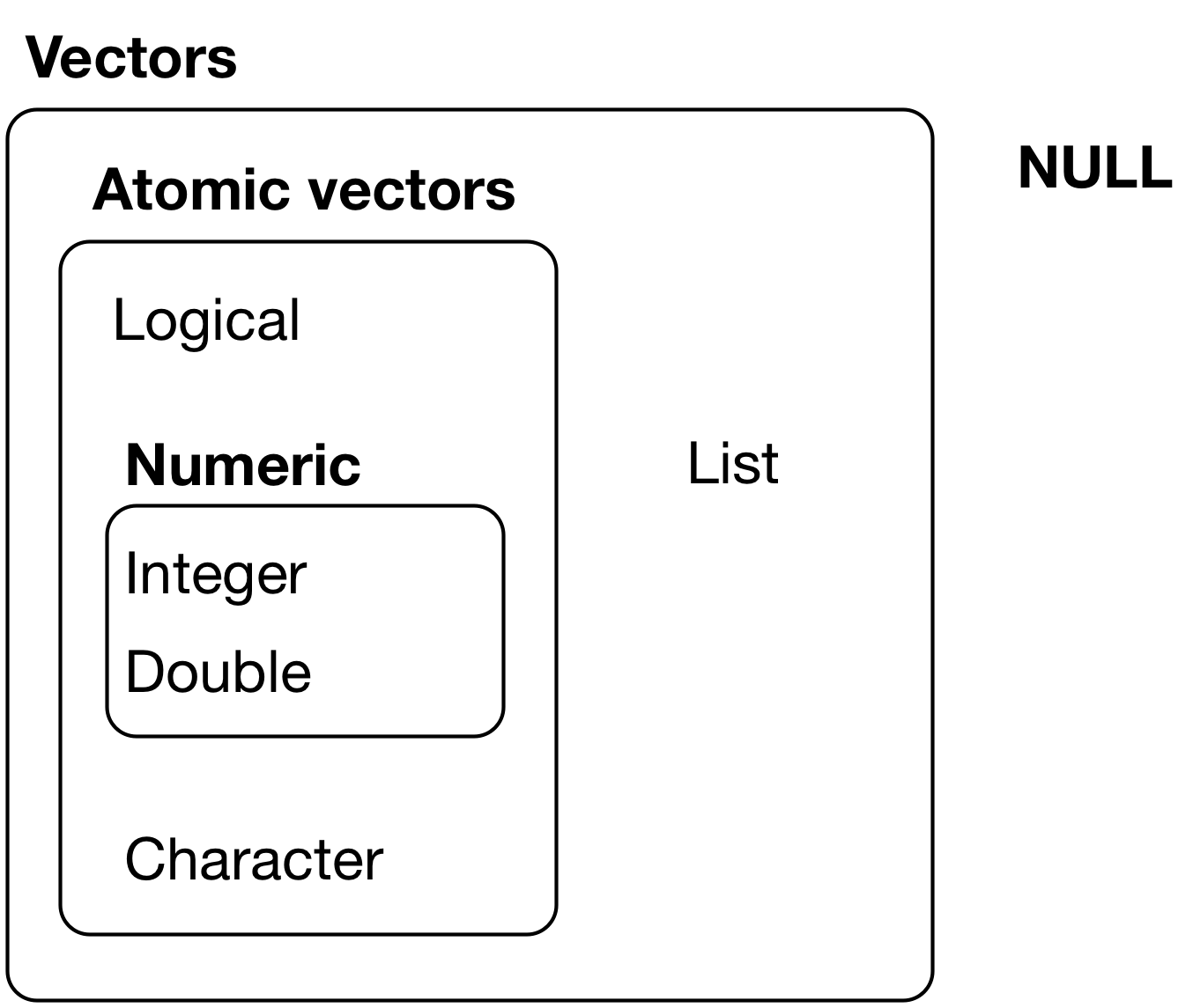
There are two types of vectors:
-
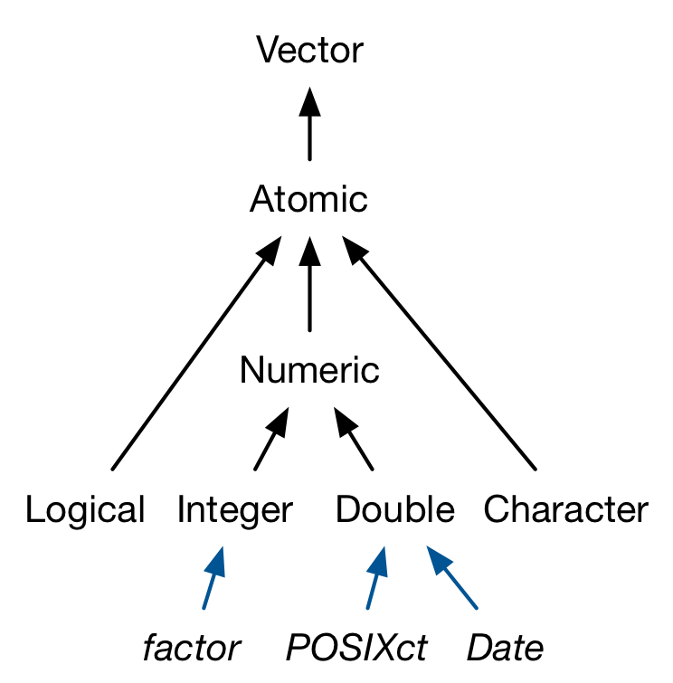
Atomic vectors, of which there are six types: logical, integer, double, character, complex, and raw. Integer and double vectors are collectively known as numeric vectors.
-
Lists, which are sometimes called recursive vectors because lists can contain other lists.
The four most important types of atomic vector are logical, integer, double, and character. Raw and complex are rarely used during a data analysis, so I won’t discuss them here.
The chief difference between atomic vectors and lists is that atomic vectors are homogeneous, while lists can be heterogeneous. There’s one other related object: NULL. NULL is often used to represent the absence of a vector (as opposed to NA which is used to represent the absence of a value in a vector). NULL typically behaves like a vector of length 0. NULL is not a vector, but often serves the role of a generic 0-length vector. Figure 20.1 summarises the interrelations.
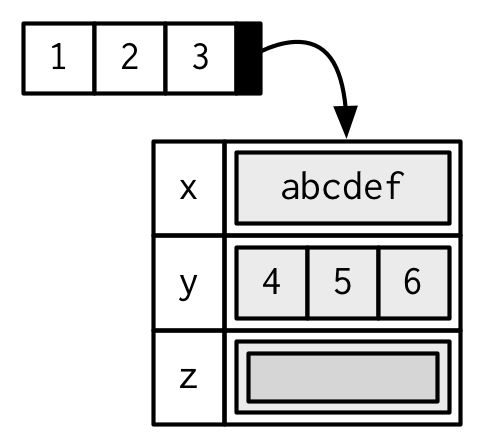
Vectors can also contain arbitrary additional metadata in the form of attributes, which you can think of as a named list containing arbitrary metadata. These attributes are used to create augmented vectors which build on additional behaviour. Two attributes are particularly important because they create important vector variants. The dimension attribute turns vectors into matrices and arrays.
The class attribute powers the S3 object system. Here you’ll learn about a handful of the most important S3 vectors: factors, date/times, data frames, and tibbles.
Matrices and data frames are not necessarily what you think of as vectors, so you’ll learn why these 2d structures are considered to be vectors in R.
There are three important types of augmented vector:
- Factors are built on top of integer vectors.
- Dates and date-times are built on top of numeric vectors.
- Data frames and tibbles are built on top of lists.
This chapter will introduce you to these important vectors from simplest to most complicated. You’ll start with atomic vectors, then build up to lists, and finish off with augmented vectors.
Character Vectors
Character vectors are the most complex type of atomic vector, because each element of a character vector is a string, and a string can contain an arbitrary amount of data.
You’ve already learned a lot about working with strings in strings. Here I wanted to mention one important feature of the underlying string implementation: R uses a global string pool. This means that each unique string is only stored in memory once, and every use of the string points to that representation. This reduces the amount of memory needed by duplicated strings.
Numeric Vectors
Integer and double vectors are known collectively as numeric vectors. In R, numbers are doubles by default. To make an integer, place an L after the number:
typeof(1)
#> [1] "double"
typeof(1L)
#> [1] "integer"
1.5L
#> [1] 1.5
The distinction between integers and doubles is not usually important, but there are two important differences that you should be aware of:
- Doubles are approximations. Doubles represent floating point numbers that can not always be precisely represented with a fixed amount of memory. This means that you should consider all doubles to be approximations. For example, what is square of the square root of two?
-
Integers have one special value:
NA, while doubles have four:NA,NaN,Infand-Inf. All three special valuesNaN,Infand-Infcan arise during division:c(-1, 0, 1) / 0 #> [1] -Inf NaN Inf
Avoid using == to check for these other special values. Instead use the helper functions is.finite(), is.infinite(), and is.nan():
| 0 | Inf | NA | NaN | |
|---|---|---|---|---|
is.finite() |
x | |||
is.infinite() |
x | |||
is.na() |
x | x | ||
is.nan() |
x |
Additional numeric vector functions
Table 6.2 contains additional functions that you will find useful when managing numeric vectors:
| Function | Description | Example | Result |
|---|---|---|---|
round(x, digits) |
Round elements in x to digits digits |
round(c(2.231, 3.1415), digits = 1) |
2.2, 3.1 |
ceiling(x), floor(x) |
Round elements x to the next highest (or lowest) integer | ceiling(c(5.1, 7.9)) |
6, 8 |
x %% y |
Modular arithmetic (ie. x mod y) | 7 %% 3 |
1 |
S3 Atomic Vectors
One of the most important attributes is class, which defines the S3 object system. Having a class attribute makes an object an S3 object, which means that it will behave differently when passed to a generic function. Every S3 object is built on top of a base type, and often stores additional information in other attributes.
In this section, we’ll discuss three important S3 vectors used in base R:
-
Categorical data, where values can only come from a fixed set of levels, are recorded in factor vectors.
-
Dates (with day resolution) are recorded in Date vectors.
-
Date-times (with second or sub-second resolution) are stored in POSIXct vectors.
Logical Vectors
Logical vectors are the simplest type of atomic vector because they can take only three possible values: FALSE, TRUE, and NA.
Logical vectors are usually constructed with comparison operators, as described in comparisons. You can also create them by hand with c():
1:10 %% 3 == 0
#>  [1] FALSE FALSE  TRUE FALSE FALSE  TRUE FALSE FALSE  TRUE FALSE

c(TRUE, TRUE, FALSE, NA)
#> [1]  TRUE  TRUE FALSE    NA
Attributes
R objects can have attributes, which are like metadata for the object. These metadata can be very useful in that they help to describe the object. For example, column names on a data frame help to tell us what data are contained in each of the columns. Some examples of R object attributes are
-
names, dimnames
-
dimensions (e.g. matrices, arrays)
-
class (e.g. integer, numeric)
-
length
-
other user-defined attributes/metadata
Three very important attributes that are used to implement fundamental parts of R are:
- Names are used to name the elements of a vector.
- Dimensions (dims, for short) make a vector behave like a matrix or array.
- Class is used to implement the S3 object oriented system.
Attributes of an object (if any) can be accessed using the attributes() function. Not all R objects contain attributes, in which case the attributes() function returns NULL.
You’ve seen names above, and we won’t cover dimensions because we don’t use matrices in this book. It remains to describe the class, which controls how generic functions work. Generic functions are key to object oriented programming in R, because they make functions behave differently for different classes of input. A detailed discussion of object oriented programming is beyond the scope of this book, but you can read more about it in Advanced R at http://adv-r.had.co.nz/OO-essentials.html#s3.
Here’s what a typical generic function looks like:
as.Date
#> function (x, ...)
#> UseMethod("as.Date")
#> <bytecode: 0x55cb1e0>
#> <environment: namespace:base>
The call to “UseMethod” means that this is a generic function, and it will call a specific method, a function, based on the class of the first argument. (All methods are functions; not all functions are methods). You can list all the methods for a generic with methods():
methods("as.Date")
#> [1] as.Date.character as.Date.default   as.Date.factor    as.Date.numeric
#> [5] as.Date.POSIXct   as.Date.POSIXlt
#> see '?methods' for accessing help and source code
For example, if x is a character vector, as.Date() will call as.Date.character(); if it’s a factor, it’ll call as.Date.factor().
The most important S3 generic is print(): it controls how the object is printed when you type its name at the console. Other important generics are the subsetting functions [, [[, and $.
All R objects can have attributes that help to describe what is in the object. Perhaps the most useful attribute is names, such as column and row names in a data frame, or simply names in a vector or list. Attributes like dimensions are also important as they can modify the behavior of objects, like turning a vector into a matrix.
Getting and setting attributes
Any vector can contain arbitrary additional metadata through its attributes. You can think of attributes as named list of vectors that can be attached to any object. You can get and set individual attribute values with attr() or see them all at once with attributes().
The function attributes(object)returns a list of all the non-intrinsic attributes currently defined for that object.
The function attr(object, name)can be used to select a specific attribute.
These functions are rarely used, except in rather special circumstances when some new attribute is being created for some particular purpose, for example to associate a creation date or an operator with an R object. The concept, however, is very important.
Some care should be exercised when assigning or deleting attributes since they are an integral part of the object system used in R.
When it is used on the left hand side of an assignment it can be used either to associate a new attribute with object or to change an existing one. For example
> attr(z, "dim") <- c(10,10)
allows R to treat z as if it were a 10-by-10 matrix.
Intrinsic attributes: mode and length
By the mode of an object we mean the basic type of its fundamental constituents. This is a special case of a “property” of an object. Another property of every object is its length. The functions mode(object) and length(object) can be used to find out the mode and length of any defined structure 11.
Further properties of an object are usually provided by attributes(object), see Getting and setting attributes. Because of this, mode and length are also called “intrinsic attributes” of an object.
For example, if z is a complex vector of length 100, then in an expression mode(z) is the character string "complex" and length(z) is 100.
R caters for changes of mode almost anywhere it could be considered sensible to do so, (and a few where it might not be). For example with
> z <- 0:9
we could put
> digits <- as.character(z)
after which digits is the character vector c("0", "1", "2",
…, "9"). A further coercion, or change of mode, reconstructs the numerical vector again:
> d <- as.integer(digits)
Now d and z are the same.12 There is a large collection of functions of the form as.something() for either coercion from one mode to another, or for investing an object with some other attribute it may not already possess. The reader should consult the different help files to become familiar with them.
With atomic vectors
You might have noticed that the set of atomic vectors does not include a number of important data structures like matrices and arrays, factors and date/times.
These types are built on top of atomic vectors by adding attributes. In this section, you’ll learn the basics of attributes, and how the dim attribute makes matrices and arrays.
Below you’ll learn how the class attribute is used to create S3 vectors, including factors, dates, and date-times.
You can think of attributes as a named list14 used to attach metadata to an object. Individual attributes can be retrieved and modified with attr(), or retrieved en masse with attributes(), and set en masse with structure().
Attributes should generally be thought of as ephemeral. For example, most attributes are lost by most operations:
attributes(a[1])
attributes(sum(a))
There are only two attributes that are routinely preserved:
-
names, a character vector giving each element a name.
-
dim, short for dimensions, an integer vector, used to turn vectors into matrices and arrays.
To preserve additional attributes, you’ll need to create your own S3 class, the topic of Chapter 12.
Names
R objects can have names, which is very useful for writing readable code and self-describing objects.
You can name a vector in three ways:
# When creating it:
x <- c(a = 1, b = 2, c = 3)

# By assigning names() to an existing vector:
x <- 1:3
names(x) <- c("a", "b", "c")

# Inline, with setNames():
x <- setNames(1:3, c("a", "b", "c"))
Avoid using attr(x, "names") as it requires more typing and is less readable than names(x). You can remove names from a vector by using unname(x) or names(x) <- NULL.
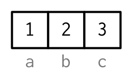
To be technically correct, when drawing the named vector x, I should draw it like so:
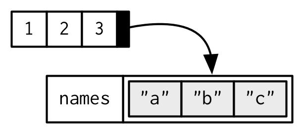 However, names are so special and so important, that unless I’m trying specifically to draw attention to the attributes data structure, I’ll use them to label the vector directly:
To be maximally useful for character subsetting (e.g. Section 4.5.1) names should be unique, and non-missing, but this is not enforced by R.
Depending on how the names are set, missing names may be either "" or NA_character_. If all names are missing, names() will return NULL.
Note that for data frames, there is a separate function for setting the row names, the row.names() function.
Also, data frames do not have column names, they just have names (like lists). So to set the column names of a data frame just use the names() function.
Yes, I know its confusing. Here’s a quick summary:
| Object | Set column names | Set row names |
|---|---|---|
| data frame | names() |
row.names() |
| matrix | colnames() |
rownames() |
Dimensions
Adding a dim attribute to a vector allows it to behave like a 2-dimensional matrix or multi-dimensional array.
Matrices and arrays are primarily a mathematical/statistical tool, not a programming tool, so will be used infrequently in this book, and only covered briefly. Their most important feature is multidimensional subsetting, which is covered in Section 4.2.3.
You can create matrices and arrays with matrix() and array(), or by using the assignment form of dim().
Many of the functions for working with vectors have generalisations for matrices and arrays:
| Vector | Matrix | Array |
|---|---|---|
names() |
rownames(), colnames() |
dimnames() |
length() |
nrow(), ncol() |
dim() |
c() |
rbind(), cbind() |
abind::abind() |
| — | t() |
aperm() |
is.null(dim(x)) |
is.matrix() |
is.array() |
A vector without dim attribute set is often thought of as 1-dimensional, but actually has a NULL dimensions. You also can have matrices with a single row or single column, or arrays with a single dimension. They may print similarly, but will behave differently. The differences aren’t too important, but it’s useful to know they exist in case you get strange output from a function (tapply() is a frequent offender). As always, use str() to reveal the differences.
Missing values
Missing values are denoted by NA or NaN for q undefined mathematical operations.
-
is.na()is used to test objects if they areNA -
is.nan()is used to test forNaN -
NAvalues have a class also, so there are integerNA, characterNA, etc. -
A
NaNvalue is alsoNAbut the converse is not true
Note that each type of atomic vector has its own missing value:
NA            # logical
#> [1] NA
NA_integer_   # integer
#> [1] NA
NA_real_      # double
#> [1] NA
NA_character_ # character
#> [1] NA
Normally you don’t need to know about these different types because you can always use NA and it will be converted to the correct type using the implicit coercion rules described next. However, there are some functions that are strict about their inputs, so it’s useful to have this knowledge sitting in your back pocket so you can be specific when needed.