Chapter 2.2.2 Subsetting
Introduction
R’s subsetting operators are powerful and fast. Mastery of subsetting allows you to succinctly express complex operations in a way that few other languages can match. Subsetting is easy to learn but hard to master because you need to internalise a number of interrelated concepts:
-
The six types of thing that you can subset with.
-
The three subsetting operators,
[[,[, and$. -
How the subsetting operators interact with vector types (e.g., atomic vectors, lists, factors, matrices, and data frames).
-
The use of subsetting together with assignment.
This chapter helps you master subsetting by starting with the simplest type of subsetting: subsetting an atomic vector with [. It then gradually extends your knowledge, first to more complicated data types (like arrays and lists), and then to the other subsetting operators, [[ and $. You’ll then learn how subsetting and assignment can be combined to modify parts of an object, and, finally, you’ll see a large number of useful applications.
Subsetting is a natural complement to str(). str() shows you the structure of any object, and subsetting allows you to pull out the pieces that you’re interested in. For large, complex objects, I also highly recommend the interactive RStudio Viewer, which you can activate with View(my_object).
Atomic Vectors
This section starts by teaching you about [. You’ll start by learning the six types of data that you can use to subset atomic vectors. You’ll then learn how those six data types act when used to subset lists, matrices, and data frames.
It’s easiest to learn how subsetting works for atomic vectors, and then how it generalises to higher dimensions and other more complicated objects.
We’ll start with [, the most commonly used operator which allows you to extract any number of elements.
[ is the subsetting function, and is called like x[a]. There are four types of things that you can subset a vector with:
-
A numeric vector containing only integers. The integers must either be all positive, all negative, or zero. Subsetting with positive integers keeps the elements at those positions.
- Subsetting with a logical vector keeps all values corresponding to a
TRUEvalue. This is most often useful in conjunction with the comparison functions. - If you have a named vector, you can subset it with a character vector:
- The simplest type of subsetting is nothing,
x[], which returns the completex. This is not useful for subsetting vectors, but it is useful when subsetting matrices (and other high dimensional structures) because it lets you select all the rows or all the columns, by leaving that index blank. For example, ifxis 2d,x[1, ]selects the first row and all the columns, andx[, -1]selects all rows and all columns except the first.
There is an important variation of [ called [[. [[ only ever extracts a single element, and always drops names. It’s a good idea to use it whenever you want to make it clear that you’re extracting a single item, as in a for loop. The distinction between [ and [[ is most important for lists, as we’ll see shortly. The next section will cover [[ and $, used to extract a single element from a data structure.
Lists
Subsetting a list works in the same way as subsetting an atomic vector. Using [ will always return a list; [[ and $, as described in Section 4.3, let you pull out the components of the list.
Data Frames and Tibbles
you can subset a data frame or a tibble like a 1d structure (where it behaves like a list), or a 2d structure (where it behaves like a matrix).
Data frames possess the characteristics of both lists and matrices: if you subset with a single vector, they behave like lists; if you subset with two vectors, they behave like matrices.
In my opinion, data frames have two suboptimal subsetting behaviours:
-
When you subset columns with
df[, vars], you will get a vector ifvarsselects one variable, otherwise you’ll get a data frame. This is a frequent source of bugs when using[in a function, unless you always remember to dodf[, vars, drop = FALSE]. -
When you attempt to extract a single column with
df$xand there is no columnx, a data frame will instead select any variable that starts withx. If no variable starts withx,df$xwill returnNULL. This makes it easy to select the wrong variable or to select a variable that doesn’t exist.
Tibbles tweak these behaviours so that [ always returns a tibble, and $ doesn’t partial match, and warns if it can’t find a variable (this is what makes tibbles surly).
So far we’ve used dplyr::filter() to filter the rows in a tibble. filter() only works with tibble, so we’ll need a new tool for vectors: [.
A tibble’s insistence on returning a data frame from [ can cause problems with legacy code, which often uses df[, "col"] to extract a single column. To fix this, use df[["col"]] instead; this is more expressive (since [[ always extracts a single element) and works with both data frames and tibbles.
Matrices and Arrays
You can subset higher-dimensional structures in three ways:
- With multiple vectors.
- With a single vector.
- With a matrix.
The most common way of subsetting matrices (2d) and arrays (>2d) is a simple generalisation of 1d subsetting: you supply a 1d index for each dimension, separated by a comma. Blank subsetting is now useful because it lets you keep all rows or all columns.
By default, [ will simplify the results to the lowest possible dimensionality. You’ll learn how to avoid this in Section 4.2.5.
Because matrices and arrays are just vectors with special attributes, you can subset them with a single vector, as if they were a 1d vector. Arrays in R are stored in column-major order.
You can also subset higher-dimensional data structures with an integer matrix (or, if named, a character matrix). Each row in the matrix specifies the location of one value, where each column corresponds to a dimension in the array being subsetted. This means that you use a 2 column matrix to subset a matrix, a 3 column matrix to subset a 3d array, and so on. The result is a vector of values.
Preserving Dimensionality
By default, any subsetting 2d data structures with a single number, single name, or a logical vector containing a single TRUE will simplify the returned output, i.e. it will return an object with lower dimensionality. To preserve the original dimensionality, you must use drop = FALSE
-
For matrices and arrays, any dimensions with length 1 will be dropped:
-
Data frames with a single column will return just that column:
-
Tibbles default to
drop = FALSE, and[will never return a single vector.
The default drop = TRUE behaviour is a common source of bugs in functions: you check your code with a data frame or matrix with multiple columns, and it works. Six months later you (or someone else) uses it with a single column data frame and it fails with a mystifying error. When writing functions, get in the habit of always using drop = FALSE when subsetting a 2d object.
Factor subsetting also has a drop argument, but the meaning is rather different. It controls whether or not levels are preserved (not the dimensionality), and it defaults to FALSE (levels are preserved, not simplified by default). If you find you are using drop = TRUE a lot it’s often a sign that you should be using a character vector instead of a factor.
Subsetting and assignment
All subsetting operators can be combined with assignment to modify selected values of the input vector.
Subsetting with nothing can be useful in conjunction with assignment because it will preserve the structure of the original object. Compare the following two expressions. In the first, mtcars will remain as a data frame. In the second, mtcars will become a list.
mtcars[] <- lapply(mtcars, as.integer)
mtcars <- lapply(mtcars, as.integer)
Selecting a single element - [[
There are two other subsetting operators: [[ and $.
[[ is used for extracting single items,
and x$y is a useful shorthand for x[["y"]].
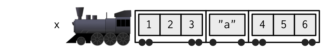
[[ is most important working with lists because subsetting a list with [ always returns a smaller list. To help make this easier to understand we can use a metaphor:
“If list
xis a train carrying objects, thenx[[5]]is the object in car 5;x[4:6]is a train of cars 4-6.”— @RLangTip, https://twitter.com/RLangTip/status/268375867468681216
Let’s make a simple list and draw it as a train:
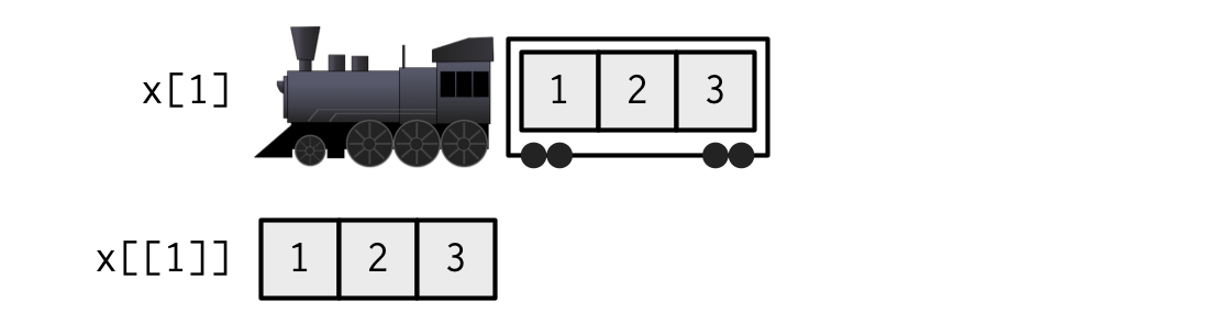
When extracting a single element, you have two options: you can create a smaller train, or you can extract the contents of a carriage. This is the difference between
[and[[:
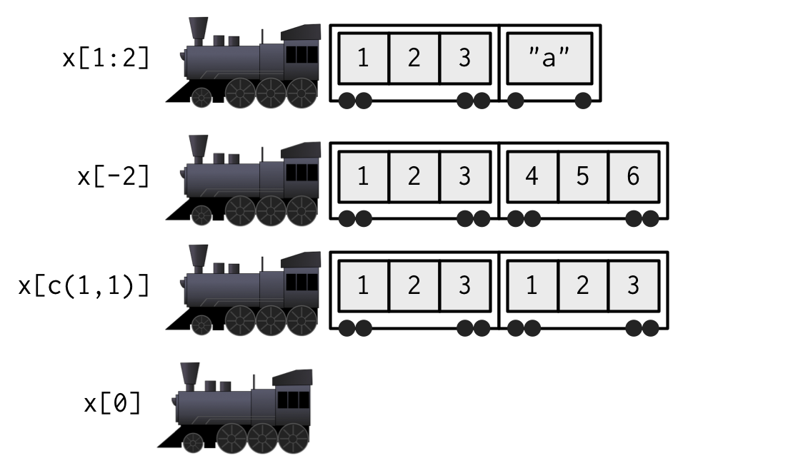
When extracting multiple elements (or zero!), you have to make a smaller train:
Missing/out of bounds indices
It’s useful to understand what happens with [ and [[ when you use an “invalid” index. The following tables summarise what happens when you subset a logical vector, list, and NULL with an out-of-bounds value (OOB), a missing value (e.g. NA_integer_), and a zero-length object (like NULL or logical()) with [ and [[. Each cell shows the result of subsetting the data structure named in the row by the type of index described in the column. I’ve only shown the results for logical vectors, but other atomic vectors behave similarly, returning elements of the same type.
row[col] |
Zero-length | OOB | Missing |
|---|---|---|---|
NULL |
NULL |
NULL |
NULL |
| Logical | logical(0) |
NA |
NA |
| List | list() |
list(NULL) |
list(NULL) |
With [, it doesn’t matter whether the OOB index is a position or a name, but it does for [[:
row[[col]] |
Zero-length | OOB (int) | OOB (chr) | Missing |
|---|---|---|---|---|
NULL |
NULL |
NULL |
NULL |
NULL |
| Atomic | Error | Error | Error | Error |
| List | Error | Error | NULL |
NULL |
If the input vector is named, then the names of OOB, missing, or NULL components will be "<NA>".
The inconsistency of the [[ table above lead to the development of purrr::pluck() and purrr::chuck(). pluck() always returns NULL (or the value of the .default argument) when the element is missing; chuck() always throws an error:
pluck(row, col) |
Zero-length | OOB (int) | OOB (chr) | Missing |
|---|---|---|---|---|
NULL |
NULL |
NULL |
NULL |
NULL |
| Atomic | NULL |
NULL |
NULL |
NULL |
| List | NULL |
NULL |
NULL |
NULL |
chuck(row, col) |
Zero-length | OOB (int) | OOB (chr) | Missing |
|---|---|---|---|---|
NULL |
Error | Error | Error | Error |
| Atomic | Error | Error | Error | Error |
| List | Error | Error | Error | Error |
The behaviour of pluck() makes it well suited for indexing into deeply nested data structures where the component you want does not always exist (as is common when working with JSON data from web APIs). pluck() also allows you to mingle integer and character indexes, and to provide an alternative default value if the item does not exist:
$
$ is a shorthand operator:
x$y is roughly equivalent to x[["y"]].
It’s often used to access variables in a data frame, as in mtcars$cyl or diamonds$carat. One common mistake with $ is to use it when you have the name of a column stored in a variable.
@ and slot()
There are also two additional subsetting operators that are needed for S4 objects: @(equivalent to$), and slot()(equivalent to [[). @ is more restrictive than $ in that it will return an error if the slot does not exist. These are described in more detail in S4.
Applications
The basic principles described above give rise to a wide variety of useful applications. Some of the most important are described below. Many of these basic techniques are wrapped up into more concise functions (e.g., subset(), merge(), dplyr::arrange()), but it is useful to understand how they are implemented with basic subsetting. This will allow you to adapt to new situations not handled by existing functions.
Lookup tables (character subsetting)
Character matching provides a powerful way to make lookup tables. Say you want to convert abbreviations:
x <- c("m", "f", "u", "f", "f", "m", "m")
lookup <- c(m = "Male", f = "Female", u = NA)
lookup[x]
#>        m        f        u        f        f        m        m
#>   "Male" "Female"       NA "Female" "Female"   "Male"   "Male"

unname(lookup[x])
#> [1] "Male"   "Female" NA       "Female" "Female" "Male"   "Male"
If you don’t want names in the result, use unname() to remove them.
Matching and merging by hand (integer subsetting)
You may have a more complicated lookup table which has multiple columns of information. Suppose we have a vector of integer grades, and a table that describes their properties:
grades <- c(1, 2, 2, 3, 1)

info <- data.frame(
  grade = 3:1,
  desc = c("Excellent", "Good", "Poor"),
  fail = c(F, F, T)
)
Random samples/bootstraps (integer subsetting)
You can use integer indices to perform random sampling or bootstrapping of a vector or data frame. sample() generates a vector of indices, then subsetting accesses the values.
The arguments of sample() control the number of samples to extract, and whether sampling is performed with or without replacement.
Ordering (integer subsetting)
order() takes a vector as input and returns an integer vector describing how the subsetted vector should be ordered:
To break ties, you can supply additional variables to order(), and you can change from ascending to descending order using decreasing = TRUE. By default, any missing values will be put at the end of the vector; however, you can remove them with na.last = NA or put at the front with na.last = FALSE.
For two or more dimensions, order() and integer subsetting makes it easy to order either the rows or columns of an object.
Expanding aggregated counts (integer subsetting)
Sometimes you get a data frame where identical rows have been collapsed into one and a count column has been added. rep() and integer subsetting make it easy to uncollapse the data by subsetting with a repeated row index.
Removing columns from data frames (character subsetting)
There are two ways to remove columns from a data frame. You can set individual columns to NULL:
df <- data.frame(x = 1:3, y = 3:1, z = letters[1:3])
df$z <- NULL
Or you can subset to return only the columns you want:
df <- data.frame(x = 1:3, y = 3:1, z = letters[1:3])
df[c("x", "y")]
#> x y
#> 1 1 3
#> 2 2 2
#> 3 3 1
If you only know the columns you don’t want, use set operations to work out which columns to keep:
df[setdiff(names(df), "z")]
#> x y
#> 1 1 3
#> 2 2 2
#> 3 3 1
Selecting rows based on a condition (logical subsetting)
Because it allows you to easily combine conditions from multiple columns, logical subsetting is probably the most commonly used technique for extracting rows out of a data frame.
Remember to use the vector boolean operators & and |, not the short-circuiting scalar operators && and || which are more useful inside if statements. Don’t forget De Morgan’s laws, which can be useful to simplify negations:
!(X & Y)is the same as!X | !Y!(X | Y)is the same as!X & !Y
For example, !(X & !(Y | Z)) simplifies to !X | !!(Y|Z), and then to !X | Y | Z.
Boolean algebra vs. sets (logical & integer subsetting)
It’s useful to be aware of the natural equivalence between set operations (integer subsetting) and boolean algebra (logical subsetting).
Using set operations is more effective when:
-
You want to find the first (or last)
TRUE. -
You have very few
TRUEs and very manyFALSEs; a set representation may be faster and require less storage.
which() allows you to convert a boolean representation to an integer representation. There’s no reverse operation in base R but we can easily create one.
When first learning subsetting, a common mistake is to use x[which(y)] instead of x[y]. Here the which() achieves nothing: it switches from logical to integer subsetting but the result will be exactly the same. In more general cases, there are two important differences.
-
When the logical vector contains
NA, logical subsetting replaces these values byNAwhilewhich()drops these values. It’s not uncommon to usewhich()for this side-effect, but that’s -
x[-which(y)]is not equivalent tox[!y]: ifyis all FALSE,which(y)will beinteger(0)and-integer(0)is stillinteger(0), so you’ll get no values, instead of all values.
In general, avoid switching from logical to integer subsetting unless you want, for example, the first or last TRUE value.