Chapter 6.1 HT and CIs For the Mean

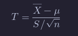
If $X1,\dots,Xn$ are iid normal rv’s with mean $μ$ and standard deviation $σ$ , then $X¯$ is normal with mean $μ$ and standard deviation $σ/sqrt{n}$ . Then

X¯-μ/σ/sqrt{n} ~ Z

where $Z$ is standard normal. One can use this information to do computations about probabilities of $X¯$ in the case when $σ$ is known. However, many times, $σ$ is not known. In that case, we replace $σ$ by its estimate based on the data, $S$ . The value $S/sqrt{n}$ is called the standard error of $X¯$ . The standard error is no longer the standard deviation of $X¯$ , but an approximation that is also a random variable.

The question then becomes: what kind of distribution is X¯−μ/ S/sqrt{n} ?

Theorem

X1,\dots,Xn

are iid normal rvs with mean

μ

and sd

σ

, then

X¯-μ / S/sqrt{n}

t

with

n-1

degrees of freedom.

We will not prove this theorem, but let’s verify through simulation that the pdfs look similar in some special cases.

Now, suppose that we don’t know either $μ$ or $σ$ , but we do know that our data is randomly sampled from a normal distribution. Let $tα$ be the unique real number such that $P(t>tα)=α$ , where $t$ has $n-1$ degrees of freedom. Note that $tα$ depends on $n$ , because the $t$ distribution has more area in its tails when $n$ is small.

Then, we know that

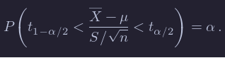
By rearranging, we get

Because the $t$ distribution is symmetric, $t1-α/2=-tα/2$ , so we can rewrite the equation symmetrically as:

Let’s think about what this means. Take n=10 and α=0.10 just to be specific. This means that if I were to repeatedly take 10 samples from a normal distribution with mean μ and any σ, then 90% of the time, μ would lie between $X¯+tα/2S/sqrt{n}$ and $X¯-tα/2S/sqrt{n}$ . That sounds like something that we need to double check using a simulation!

Summary

To review, these are the steps one would take whenever you’d like to do a hypothesis test comparing values from the distributions of two groups:

Simulate many samples using a random process that matches the way the original data were collected and that assumes the null hypothesis is true.

Collect the values of a sample statistic for each sample created using this random process to build a null distribution.

Assess the significance of the original sample by determining where its sample statistic lies in the null distribution.

If the proportion of values as extreme or more extreme than the observed statistic in the randomization distribution is smaller than the pre-determined significance level α, we reject H0. Otherwise, we fail to reject H0. (If no significance level is given, one can assume α=0.05.)

Confidence intervals for the mean

If we take a sample of size $n$ from iid normal random variables, then we call the interval

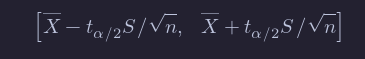
a 100(1 - $α$ )% confidence interval for $μ$ .

As we saw in the simulation above, what this means is that if we repeat this experiment many times, then in the limit 100(1 - $α$ )% of the time, the mean $μ$ will lie in the confidence interval.

Of course, once we have done the experiment and we have an interval, it doesn’t make sense to talk about the probability that $μ$ (a constant) is in the (constant) interval. There is nothing random there. However, we can say that we are 100(1 - $α$ )% confident that the mean is in the interval.

As you might imagine, R has a built in command that does all of this for us. Consider the heart rate and body temperature data normtemp.⁵

We see that the data set is 130 observations of body temperature and heart rate. There is also gender information attached, that we will ignore for the purposes of this example.

Let’s find a 98 confidence interval for the mean heart rate of healthy adults. In order for this to be valid, we are assuming that we have a random sample from all healthy adults (highly unlikely to be formally true), and that the heart rate of healthy adults is normally distributed (also unlikely to be formally true). Later, we will discuss deviations from our assumptions and when we should be concerned.

The R command that finds a confidence interval for the mean in this way is

t.test(normtemp$Heart.Rate, conf.level = .98)

## 
##  One Sample t-test
## 
## data:  normtemp$Heart.Rate
## t = 119.09, df = 129, p-value < 2.2e-16
## alternative hypothesis: true mean is not equal to 0
## 98 percent confidence interval:
##  72.30251 75.22056
## sample estimates:
## mean of x 
##  73.76154

We get a lot of information, but we can pull out what we are looking for as the confidence interval [72.3, 75.2]. So, we are 98 confident that the mean heart rate of healthy adults is greater than 72.3 and less than 75.2.

NOTE We are not saying anything about the mean heart rate of the people in the study. That is exactly 73.76154, and we don’t need to do anything fancy. We are making an inference about the mean heart rate of all healthy adults.

Note that to be more precise, we might want to say it is the mean heart rate of all healthy adults as would be measured by this experimenter. Other experimenters could have a different technique for measuring hear rates which would lead to a different answer. It is traditional to omit that statement from conclusions, though you might consider its implications in the following exercise.

One-sided Confidence Intervals and Hypothesis Tests

Consider the data set anorexia, in the MASS library. Since we do not need the entire MASS package and MASS has a function select that interferes with the dplyr function that we use a lot, let’s just load the data from MASS into a variable called anorexia without loading the entire MASS package.

anorexia <- MASS::anorexia

This data set consists of pre- and post- treatment measurements for anorexia patients. There are three different treatments of patients, which we ignore in this example (we will come back to that later in the class). In this case, we have reason to believe that the medical treatment that the patients are undergoing will result in an increased weight. So, we are not as much interested in detecting a change in weight, but an increase in weight. This changes our analysis.

We will construct a 98% confidence interval for the variable weight difference of the form $(L,\infty)$ . We will say that we are 98% confident that the treatment results in a mean change of weight of at least $L$ pounds. As before, this interval will be constructed so that 98% of the time that we perform the experiment, the true mean will fall in the interval (and 2% of the time, it will not). As before, we are assuming normality of the underlying population. We will also perform the following hypothesis test:

$H0:μ\leq0$ vs

$Ha:μ>0$

There is no practical difference between $H0:μ\leq0$ and $H0:μ=0$ in this case, but knowing the alternative is $μ>0$ makes a difference. Now, the evidence that is most in favor of $Ha$ is all of the form $x¯>L\overline{x} > L$ . So, the percent of time we would make a type I error under $H0H_0$ is

P(X¯−μ0S/n>L)P(\frac{\overline{X} - \mu_0}{S/\sqrt{n}} > L)

where $μ0=0\mu_0 = 0$ in this case. After collecting data, if we reject $H0H_0$ , we would also have rejected $H0H_0$ if we got more compelling evidence against $H0H_0$ , so we would compute

P(tn−1>x¯−μ0S/n)P(t_{n-1} > \frac{\overline{x} - \mu_0}{S/\sqrt{n}})

where $x¯−μ0S/n\frac{\overline{x} - \mu_0}{S/\sqrt{n}}$ is the value computed from the data.

Skew

...

Note that we have to specify the null hypothesis mu = 1 in the t.test. Here we get an effective type I error rate (rejecting $H_{0}$ when $H_{0}$ is true) that is 3.035 percentage points higher than designed. This means our error rate will increase by 61%. Most people would argue that the test is not working as designed.

One issue is the following: how do we know we have run replicate enough times to get a reasonable estimate for the probability of a type I error? Well, we don’t. If we repeat our experiment a couple of times, though, we see that we get consistent results, which for now we will take as sufficient evidence that our estimate is closer to correct.

From the previous exercise, you should be able to see that at $n = 50$ , the effective type I error rate gets worse in relative terms as $α$ gets smaller. (For example, my estimate at the $α = .001$ level is an effective error rate more than 6 times what is designed! We would all agree that the test is not performing as designed.) That is unfortunate, because small $α$ are exactly what we are interested in! That’s not to say that t-tests are useless in this context, but $p$ -values should be interpreted with some level of caution when there is thought that the underlying population might be exponential. In particular, it would be misleading to report a $p$ -value with 7 significant digits in this case, as R does by default, when in fact it is only the order of magnitude that is significant. Of course, if you know your underlying population is exponential before you start, then there are techniques that you can use to get accurate results which are beyond the scope of this textbook.

Summary

When doing t-tests on populations that are not normal, the following types of departures from design were noted.

When the underlying distribution is skew, the exact $p$ -values should not be reported to many significant digits (especially the smaller they get). If a $p$ -value close to the $α$ level of a test is obtained, then we would want to note the fact that we are unsure of our $p$ -values due to skewness, and fail to reject.

When the underlying distribution has outliers, the power of the test is severely compromised. A single outlier of sufficient magnitude will force a t-test to never reject the null hypothesis. If your population has outliers, you do not want to use a t-test.

Tabular Data

Test of proportions

Many times, we are interested in estimating and inference on the proportion $p$ in a Bernoulli trial. For example, we may be interested in the true proportion of times that a die shows a 6 when rolled, or the proportion of voters in a population who favor a particular candidate. In order to do this, we will run $n$ trials of the experiment and count the number of times that the event in question occurs, which we denote by $x$ . For example, we could toss the die $n = 100$ times and count the number of times that a 6 occurs, or sample $n = 500$ voters (from a large population) and ask them whether they prefer a particular candidate. Note that in the second case, this is not formally a Bernoulli trial unless you allow the possibility of asking the same person twice; however, if the population is large, then it is approximately repeated Bernoulli trials.

The natural estimator for the true proportion $p$ is given by $^p = \frac{x/}{n.}$ However, we would like to be able to form confidence intervals and to do hypothesis testing with regards to $p$ . Here, we present the theory associated with performing exact binomial hypothesis tests using binom.test, as well as prop.test, which uses the normal approximation.

HTs of the Mean

Basics of hypothesis testing

In a hypothesis test, we will use data from a sample to help us decide between two competing hypotheses about a population. We make these hypotheses more concrete by specifying them in terms of at least one population parameter of interest.

We refer to the competing claims about the population as the null hypothesis, denoted by $H_{0}$ , and the alternative (or research) hypothesis, denoted by $H_{a}$ . The roles of these two hypotheses are NOT interchangeable. In a hypothesis test, we make a statement about which one might be true, but we might choose incorrectly.

The claim for which we seek significant evidence is assigned to the alternative hypothesis. The alternative is usually what the experimenter or researcher wants to establish or find evidence for.
The alternative hypothesis states that the null hypothesis is false, sometimes in a particular way.
Usually, the null hypothesis is a claim that there really is “no effect” or “no difference.” In many cases, the null hypothesis represents the status quo or that nothing interesting is happening. It can take on several forms: that a population is a specified value, that two population parameters are equal, that two population distributions are equal, and many others. The common thread being that it is a statement about the population distribution. Typically, the null hypothesis is the default assumption, or the conventional wisdom about a population. Often it is exactly the thing that a researcher is trying to show is false.
We assess the strength of evidence by assuming the null hypothesis is true and determining how unlikely it would be to see sample results/statistics as extreme (or more extreme) as those in the original sample.

Consider as an example, the body temperature of healthy adults, as in the previous subsection. The natural choice for the null and alternative hypothesis is

$H0:μ=98.6$ versus

$Ha:μ\neq98.6$ .

We will either reject $H0$ in favor of $Ha$ , or we will not reject $H0$ in favor of $Ha$ . (Note that this is different than accepting $H0$ .)

Hypothesis testing brings about many weird and incorrect notions in the scientific community and society at large. One reason for this is that statistics has traditionally been thought of as this magic box of algorithms and procedures to get to results and this has been readily apparent if you do a Google search of “flowchart statistics hypothesis tests”. There are so many different complex ways to determine which test is appropriate.

You’ll see that we don’t need to rely on these complicated series of assumptions and procedures to conduct a hypothesis test any longer. These methods were introduced in a time when computers weren’t powerful. Your cellphone (in 2016) has more power than the computers that sent NASA astronauts to the moon after all. We’ll see that ALL hypothesis tests can be broken down into the following framework given by Allen Downey here:

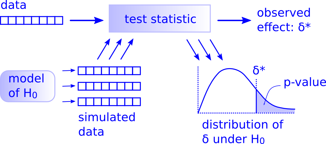
Figure 10.1: Hypothesis Testing Framework

Before we hop into this framework, we will provide another way to think about hypothesis testing that may be useful.

In the last two sections, we utilized a hypothesis test, which is a formal technique for evaluating two competing possibilities. In each scenario, we described a null hypothesis, which represented either a skeptical perspective or a perspective of no difference. We also laid out an alternative hypothesis, which represented a new perspective such as the
possibility that there has been a change or that there is a treatment effect in an experiment.

Logic of hypothesis testing

Take a random sample (or samples) from a population (or multiple populations)
If the sample data are consistent with the null hypothesis, do not reject the null hypothesis.
If the sample data are inconsistent with the null hypothesis (in the direction of the alternative hypothesis), reject the null hypothesis and conclude that there is evidence the alternative hypothesis is true (based on the particular sample collected).

Statistical significance

The idea that sample results are more extreme than we would reasonably expect to see by random chance if the null hypothesis were true is the fundamental idea behind statistical hypothesis tests. If data at least as extreme would be very unlikely if the null hypothesis were true, we say the data are statistically significant. Statistically significant data provide convincing evidence against the null hypothesis in favor of the alternative, and allow us to generalize our sample results to the claim about the population.

Z score in a hypothesis test

In the context of a hypothesis test, the Z score for a point estimate is

Z = (point estimate − null value) / SE

The standard error in this case is the equivalent of the standard deviation of the point estimate, and the null value comes from the null hypothesis.

Criminal trial analogy

We can think of hypothesis testing in the same context as a criminal trial in the United States. A criminal trial in the United States is a familiar situation in which a choice between two contradictory claims must be made.

The accuser of the crime must be judged either guilty or not guilty.
Under the U.S. system of justice, the individual on trial is initially presumed not guilty.
Only STRONG EVIDENCE to the contrary causes the not guilty claim to be rejected in favor of a guilty verdict.
The phrase “beyond reasonable doubt” is often used to set the cutoff value for when enough evidence has been given to convict.

Theoretically, we should never say “The person is innocent.” but instead “There is not sufficient evidence to show that the person is guilty.”

This is also the case with hypothesis testing; even if we fail to reject the null hypothesis, we typically do not accept the null hypothesis as truth. Failing to find strong evidence for the alternative hypothesis is not equivalent to providing evidence that the null hypothesis is true.

Now let’s compare that to how we look at a hypothesis test.

The decision about the population parameter(s) must be judged to follow one of two hypotheses.
We initially assume that $H_{0}$ is true.
The null hypothesis $H_{0}$ will be rejected (in favor of $H_{a}$ ) only if the sample evidence strongly suggests that $H_{0}$ is false. If the sample does not provide such evidence, $H_{0}$ will not be rejected.
The analogy to “beyond a reasonable doubt” in hypothesis testing is what is known as the significance level. This will be set before conducting the hypothesis test and is denoted as $α$ . Common values for $α$ are 0.1, 0.01, and 0.05.

Two possible conclusions

Therefore, we have two possible conclusions with hypothesis testing:

Reject $H_{0}$

Fail to reject $H_{0}$

Gut instinct says that “Fail to reject $H_{0}$ ” should say “Accept $H_{0}$ ” but this technically is not correct. Accepting $H_{0}$ is the same as saying that a person is innocent. We cannot show that a person is innocent; we can only say that there was not enough substantial evidence to find the person guilty.

When you run a hypothesis test, you are the jury of the trial. You decide whether there is enough evidence to convince yourself that $H_{a}$ is true (“the person is guilty”) or that there was not enough evidence to convince yourself $H_{a}$ is true (“the person is not guilty”). You must convince yourself (using statistical arguments) which hypothesis is the correct one given the sample information.

Important note: Therefore, DO NOT WRITE “Accept $H_{0}$ ” any time you conduct a hypothesis test. Instead write “Fail to reject $H_{0}$ .”

How to use a hypothesis test

Frame the research question in terms of hypotheses. Hypothesis tests are appropriate for research questions that can be summarized in two competing hypotheses. The null hypothesis (H0) usually represents a skeptical perspective or a perspective of no difference. The alternative hypothesis (Ha) usually represents a new view or a difference.

Collect data with an observational study or experiment. If a research question can be formed into two hypotheses, we can collect data to run a hypothesis test. If the research question focuses on associations between variables but does not concern causation, we would run an observational study. If the research question seeks a causal connection between two or more variables, then an experiment should be used.

Analyze the data. Choose an analysis technique appropriate for the data and identify the p-value. So far, we’ve only seen one analysis technique: randomization. Throughout the rest of this textbook, we’ll encounter several new methods suitable for many other contexts.

Form a conclusion. Using the p-value from the analysis, determine whether the data provide statistically significant evidence against the null hypothesis. Also, be sure to write the conclusion in plain language so casual readers can understand the results.

Decision errors

Hypothesis tests are not flawless. Just think of the court system: innocent people are sometimes wrongly convicted and the guilty sometimes walk free. Unfortunately, just as a jury or a judge can make an incorrect decision in regards to a criminal trial by reaching the wrong verdict, data can point to the wrong conclusion - there is some chance we will reach the wrong conclusion via a hypothesis test about a population parameter. As with criminal trials, this comes from the fact that we don’t have complete information, but rather a sample from which to try to infer about a population. However, what distinguishes statistical hypothesis tests from a court system is that our framework allows us to quantify and control how often the data lead us to the incorrect conclusion.

The possible erroneous conclusions in a criminal trial are

an innocent person is convicted (found guilty) or
a guilty person is set free (found not guilty).

There are two types of possible errors in a hypothesis test:

rejecting $H_{0}$ when in fact $H_{0}$ is true (Type I Error) or

failing to reject $H_{0}$ when in fact $H_{0}$ is false (Type II Error).

when $Ha$ is actually true?

The risk of error is the price researchers pay for basing an inference about a population on a sample. With any reasonable sample-based procedure, there is some chance that a Type I error will be made and some chance that a Type II error will occur.

To help understand the concepts of Type I error and Type II error, observe the following table:

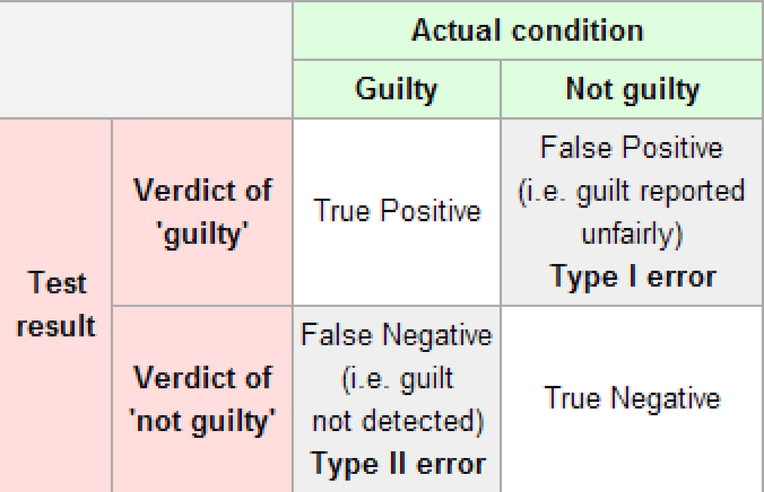
Figure 10.2: Type I and Type II errors

Conventional tests of statistical significance are based on the probability that a particular result would arise if chance alone were at work, and necessarily accept some risk of mistaken conclusions of a certain type (mistaken rejections of the null hypothesis). This level of risk is called the significance. When large numbers of tests are performed, some produce false results of this type, hence 5% of randomly chosen hypotheses turn out to be significant at the 5% level, 1% turn out to be significant at the 1% significance level, and so on, by chance alone. When enough hypotheses are tested, it is virtually certain that some will be statistically significant but misleading, since almost every data set with any degree of randomness is likely to contain (for example) some spurious correlations. If they are not cautious, researchers using data mining techniques can be easily misled by these results.

If we are using sample data to make inferences about a parameter, we run the risk of making a mistake. Obviously, we want to minimize our chance of error; we want a small probability of drawing an incorrect conclusion.

The probability of a Type I Error occurring is denoted by $α$ and is called the significance level of a hypothesis test
The probability of a Type II Error is denoted by $β$ .

Formally, we can define $α$ and $β$ in regards to the table above, but for hypothesis tests instead of a criminal trial.

$α$ corresponds to the probability of rejecting $H_{0}$ when, in fact, $H_{0}$ is true.

$β$ corresponds to the probability of failing to reject $H_{0}$ when, in fact, $H_{0}$ is false.

Ideally, we want $α = 0$ and $β = 0$ , meaning that the chance of making an error does not exist. When we have to use incomplete information (sample data), it is not possible to have both $α = 0$ and $β = 0$ . We will always have the possibility of at least one error existing when we use sample data.

Usually, what is done is that $α$ is set before the hypothesis test is conducted and then the evidence is judged against that significance level.

Common values for $α$ are 0.05, 0.01, and 0.10. If $α = 0.05$ , we are using a testing procedure that, used over and over with different samples, rejects a TRUE null hypothesis five percent of the time.

So if we can set $α$ to be whatever we want, why choose 0.05 instead of 0.01 or even better 0.0000000000000001? Well, a small $α$ means the test procedure requires the evidence against $H_{0}$ to be very strong before we can reject $H_{0}$ . This means we will almost never reject $H_{0}$ if $α$ is very small. If we almost never reject $H_{0}$ , the probability of a Type II Error – failing to reject $H_{0}$ when we should – will increase!

Thus, as $α$ decreases, $β$ increases and as $α$ increases, $β$ decreases. We, therefore, need to strike a balance in $α$ and $β$ and the common values for $α$ of 0.05, 0.01, and 0.10 usually lead to a nice balance.

For now, we will worry about controlling the probability of a Type I error.

In order to compute the probability of a type I error, we imagine that we collect the same type of data many times, when $H0$ is actually true. If we decide on rejecting $H0$ whenever it falls in a certain rejection region (RR), then the probability of a type I error would be the probability that the data falls in the rejection region given that $H0$ is true.

Making a Type 1 Error in the example's context would mean that reminding students that money not spent now can be spent later does not affect their buying habits, despite the strong evidence (the data suggesting otherwise) found in the experiment. Notice that this does not necessarily mean something was wrong with the data or that we made a computational mistake. Sometimes data simply point us to the wrong
conclusion, which is why scientific studies are often repeated to check initial findings. The example and guided practice above provide an important lesson: if we reduce how often we make one type of error, we generally make more of the other type.

Simulations

In the chapter up to this point, we have assumed that the underlying data is a random sample from a normal distribution. Let’s look at how various types of departures from that assumption affect the validity of our statistical procedures.

For the purposes of this discussion, we will restrict to hypothesis testing at a specified $α$ level, but our results will hold for confidence intervals and reporting $p$ -values just as well.

Our point of view is that if we design our hypothesis test at the $α = .1$ level, say, then we want to incorrectly reject the null hypothesis 10% of the time. That is how our test is designed.

If our assumptions of normality are violated, then we want to measure the new effective type I error rate and compare it to 10%. If the new error rate is far from 10%, then the test is not performing as designed. We will note whether the test makes too many type I errors or too few, but the main objective is to see whether the test is performing as designed.

Our first observation is that when the sample size is large, then the central limit theorem tells us that $\bar{X}$ is approximately normal. Since $t_{n}$ is also approximately normal when $n$ is large, this gives us some measure of protection against departures from normality in the underlying population. It will be very useful to pull out the $p$ -value of the t.test. Let’s see how we can do that. We begin by doing a t.test on “garbage data” just to see what t.test returns.

Choosing a significance level

Choosing a significance level for a test is important in many contexts, and the traditional level is 0.05. However, it is sometimes helpful to adjust the significance level based on the application. We may select a level that is smaller or larger than 0.05 depending on the consequences of any conclusions reached from the test.

If making a Type 1 Error is dangerous or especially costly, we should choose a small significance level (e.g. 0.01 or 0.001). Under this scenario, we want to be very cautious about rejecting the null hypothesis, so we demand very strong evidence favoring the alternative Ha before we would reject H0.

If a Type 2 Error is relatively more dangerous or much more costly than a Type 1 Error, then we should choose a higher significance level (e.g. 0.10). Here we want to be cautious about failing to reject H 0 when the null is actually false.

Significance levels should reflect consequences of errors

The significance level selected for a test should reflect the real-world consequences associated with making a Type 1 or Type 2 Error.

Let’s look at another example. Altman (1991) measured the daily energy (KJ) intake of 11 women. Let’s store it in

library(ISwR)
daily.intake <- intake$pre

It is recommended that women consume 7725 KJ per day. Is there evidence to suggest that women do not consume the recommended amount? Find a 99% confidence interval for the daily energy intake of women.

We need to assume that this is a random sample of 11 women from some population. We are making statements about the group of women that these 11 were sampled from. If they were 11 randomly selected patients of Dr.~Altman, then we are making statements about patients of Dr.~Altman. We also need to assume that energy intake is normally distributed, which seems a reasonable enough assumption. Then, we compute

t.test(daily.intake, mu = 7725, conf.level = .99)

## 
##  One Sample t-test
## 
## data:  daily.intake
## t = -2.8208, df = 10, p-value = 0.01814
## alternative hypothesis: true mean is not equal to 7725
## 99 percent confidence interval:
##  5662.256 7845.017
## sample estimates:
## mean of x 
##  6753.636

We see that the 99% confidence interval is $(5662,7845)$ , and the $p$ -value is .01814. So, there is about a 1.8% chance of getting data that is this compelling or more against $H0$ even if $H0$ is true.

We would reject $H0$ at the $α=.05$ level, but fail to reject at the $α=.01$ level. For the purposes of this book, the $α$ level will usually be specified in a problem, but if it isn’t, then you are free to choose a reasonable level based on the type of problem that we are talking about. Common choices are $α=.01$ and $α=.05$ .

p-value and statistical significance

Returning to the specifics of $H0:μ=μ0$ versus $Ha:μ\neqμ0$ , we compute the test statistic

And we ask: if I decide to reject $H0$ based on this test statistic, what percentage of the time would I get data at least that much against $H0$ even though $H0$ is true? In other words, if I decide to reject $H0$ based on $T$ , I would have to reject $H0$ for any data that is even more compelling against $H0$ . How often would that happen under $H0$ ? Well, that is what the $p$ -value is.

The p-value is the probability of observing data at least as favorable to the alternative hypothesis as our current data set, if the null hypothesis were true. We typically use a summary statistic of the data, such as a difference in proportions, to help compute the p-value and evaluate the hypotheses. This summary value that is used to compute the p-value is often called the test statistic.

When the p-value is small, i.e. less than a previously set threshold, we say the results are statistically significant. This means the data provide such strong evidence against H0 that we reject the null hypothesis in favor of the alternative hypothesis. The threshold, called the significance level and often represented by α (the Greek letter alpha), is typically set to α = 0.05, but can vary depending on the field or the application. Using a
significance level of α = 0.05 in the discrimination study, if the p-value is less than this reference value, we can say that the data provided statistically significant evidence against the null hypothesis.

I get a $p$ -value of about 0.000002, which is the probability that I would get data at least this compelling against $H0$ even though $H0$ is true.

In other words, it is very unlikely that this data would be collected if the true mean temp of healthy adults is 98.6. (Again, we are assuming a random sample of healthy adults and normal distribution of temperatures of healthy adults.)

Introducing two-sided hypotheses

So far we have explored whether women were discriminated against and whether a simple trick could make students a little thriftier. In these two case studies, we’ve actually ignored some possibilities:

• What if men are actually discriminated against?
• What if the money trick actually makes students spend more?

These possibilities weren’t considered in our hypotheses or analyses. This may have seemed natural since the data pointed in the directions in which we framed the problems.

However, there are two dangers if we ignore possibilities that disagree with our data or that conflict with our worldview:

1. Framing an alternative hypothesis simply to match the direction that the data point will generally inflate the Type 1 Error rate. After all the work we’ve done (and will continue to do) to rigorously control the error rates in hypothesis tests, careless construction of the alternative hypotheses can disrupt that hard work.

2. If we only use alternative hypotheses that agree with our worldview, then we’re going to be subjecting ourselves to confirmation bias, which means we are looking for data that supports our ideas. That’s not very scientific, and we can do better!

The previous hypotheses we’ve seen are called one-sided hypothesis tests because they only explored one direction of possibilities. Such hypotheses are appropriate when we are exclusively interested in the single direction, but usually we want to consider all possibilities.

To do so, let’s learn about two-sided hypothesis tests in the context of a new study that examines the impact of using blood thinners on patients who have undergone CPR.
Cardiopulmonary resuscitation (CPR) is a procedure used on individuals suffering a heart attack when other emergency resources are unavailable. This procedure is helpful in providing some blood circulation to keep a person alive, but CPR chest compressions can also cause internal injuries. Internal bleeding and other injuries that can result from
CPR complicate additional treatment efforts. For instance, blood thinners may be used to help release a clot that is causing the heart attack once a patient arrives in the hospital. However, blood thinners negatively affect internal injuries. Here we consider an experiment with patients who underwent CPR for a heart attack and were subsequently admitted to a hospital. 11 Each patient was randomly assigned to either receive a blood thinner (treatment group) or not receive a blood thinner (control group). The outcome variable of interest was whether the patient survived for at least 24 hours.

Example: Form hypotheses for this study in plain and statistical language. Let p c represent the true survival rate of people who do not receive a blood thinner (corresponding to the control group) and p t represent the survival rate for people receiving a blood thinner (corresponding to the treatment group).
We want to understand whether blood thinners are helpful or harmful. We’ll consider both of these possibilities using a two-sided hypothesis test.
H0 : Blood thinners do not have an overall survival effect, i.e. the survival proportions are the same in each group. p̂t − p̂c = 0.
Ha: Blood thinners have an impact on survival, either positive or negative, but not zero. p̂t − p̂c != 0.
There were 50 patients in the experiment who did not receive a blood thinner and 40 patients who did. The study results are shown in Table 2.10.

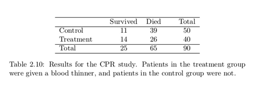
What is the observed survival rate in the control group?
And in the treatment group? Also, provide a point estimate of the difference in survival proportions of the two groups: p̂t − p̂c.

According to the point estimate, for patients who have undergone CPR outside of the hospital, an additional 13% of these patients survive when they are treated with blood thinners. However, we wonder if this difference could be easily explainable by chance.
As we did in our past two studies this chapter, we will simulate what type of differences we might see from chance alone under the null hypothesis. By randomly assigning “simulated treatment” and “simulated control” stickers to the patients’ files, we get a new grouping. If we repeat this simulation 10,000 times, we can build a null distribution of the differences shown in Figure 2.11.

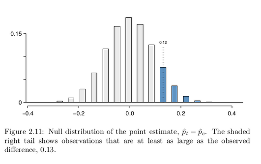
The right tail area is about 0.13. (Note: it is only a coincidence that we also have p̂t − p̂c = 0.13.) However, contrary to how we calculated the p-value in previous studies, the p-value of this test is not 0.13!

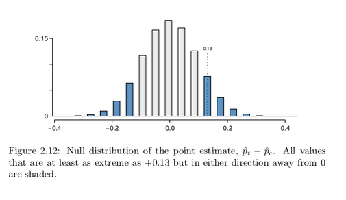
The p-value is defined as the chance we observe a result at least as favorable to the alternative hypothesis as the result (i.e. the difference) we observe. In this case, any differences less than or equal to -0.13 would also provide equally strong evidence favoring the alternative hypothesis as a difference of 0.13. A difference of -0.13 would correspond
to 13% higher survival rate in the control group than the treatment group. In Figure 2.12 we’ve also shaded these differences in the left tail of the distribution. These two shaded tails provide a visual representation of the p-value for a two-sided test.

For a two-sided test, take the single tail (in this case, 0.13) and double it to get the p-value: 0.26. Since this p-value is larger than 0.05, we do not reject the null hypothesis. That is, we do not find statistically significant evidence that the blood thinner has any influence on survival of patients who undergo CPR prior to arriving at the hospital.

Default to a two-sided test: We want to be rigorous and keep an open mind when we analyze data and evidence. Use a one-sided hypothesis test only if you truly have interest in only one direction.

Computing a p-value for a two-sided test: First compute the p-value for one tail of the distribution, then double that value to get the two-sided p-value. That’s it!

Controlling the Type 1 Error rate

It is never okay to change two-sided tests to one-sided tests after observing the data. We explore the consequences of ignoring this advice in the next example.
Example: Using α = 0.05, we show that freely switching from two-sided tests to one-sided tests will lead us to make twice as many Type 1 Errors as intended.
Suppose we are interested in finding any difference from 0. We’ve created a smooth-looking null distribution representing differences due to chance in Figure 2.13.

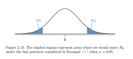
Suppose the sample difference was larger than 0. Then if we can flip to a one-sided test, we would use Ha : difference > 0. Now if we obtain any observation in the upper 5% of the distribution, we would reject H0 since the p-value would just be a the single tail. Thus, if the null hypothesis is true, we incorrectly reject the null hypothesis about 5% of the time when the sample mean is above the null value, as shown in Figure 2.13.

Suppose the sample difference was smaller than 0. Then if we change to a one-sided test, we would use H A : difference < 0. If the observed difference falls in the lower 5% of the figure, we would reject H 0 . That is, if the null hypothesis is true, then we would observe this situation about 5% of the time.

By examining these two scenarios, we can determine that we will make a Type 1 Error 5% + 5% = 10% of the time if we are allowed to swap to the “best” one-sided test for the data. This is twice the error rate we prescribed with our significance level: α = 0.05 (!).

Caution: Hypothesis tests should be set up before seeing the data:
After observing data, it is tempting to turn a two-sided test into a one-sided test. Avoid this temptation. Hypotheses should be set up before observing the data.