Chapter 2.1.1.1 Augmented Vectors
Date-times
Base R16 provides two ways of storing date-time information, POSIXct, and POSIXlt.
These are admittedly odd names: “POSIX” is short for Portable Operating System Interface, which is a family of cross-platform standards.
“ct” stands for calendar time (the time_t type in C), and “lt” for local time (the struct tm type in C).
Here we’ll focus on POSIXct, because it’s the simplest, is built on top of an atomic vector, and is most appropriate for use in data frames. POSIXct vectors are built on top of double vectors, where the value represents the number of seconds since 1970-01-01.
There is another type of date-times called POSIXlt. These are built on top of named lists:
POSIXlts are rare inside the tidyverse. They do crop up in base R, because they are needed to extract specific components of a date, like the year or month. Since lubridate provides helpers for you to do this instead, you don’t need them. POSIXct’s are always easier to work with, so if you find you have a POSIXlt, you should always convert it to a regular data time lubridate::as_date_time().
Factors
Factors are used to represent categorical data and can be unordered or ordered. They are data structures used for fields that take only predefined, finite number of values (categorical data).
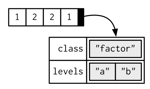
Factors are built on top of integer vectors with two attributes: the class, “factor”, which makes them behave differently from regular integer vectors, and the levels, which defines the set of allowed values.
One can think of a factor as an integer vector where each integer has a label. Using factors with labels is better than using integers because factors are self-describing. Having a variable that has values “Male” and “Female” is better than a variable that has values 1 and 2; so, the underlying representation of a variable for sex is 1:2 with labels ‘Male’ and ‘Female’. They are a special class with attributes, or metadata, that contains the information about the levels.
Factors are important in statistical modeling and are treated specially by modelling functions like lm() and glm().
Factors provide compact ways to handle categorical data.
For example, a data field such as marital status may contain only values from single, married, separated, divorced, or widowed.
In such case, we know the possible values beforehand and these predefined, distinct values are called levels. Also, you will learn about levels of a factor.
With base R15 you tend to encounter factors very frequently, because many base R functions (like read.csv() and data.frame()) automatically convert character vectors to factors. This is suboptimal, because there’s no way for those functions to know the set of all possible levels or their optimal order: the levels are a property of the experimental design, not the data. Instead, use the argument stringsAsFactors = FALSE to suppress this behaviour, and then manually convert character vectors to factors using your knowledge of the data. To learn about the historical context of this behaviour, I recommend stringsAsFactors: An unauthorized biography by Roger Peng, and stringsAsFactors = <sigh> by Thomas Lumley.
While factors look like (and often behave like) character vectors, they are built on top of integers. Be careful when treating them like strings. Some string methods (like gsub() and grepl()) will coerce factors to strings automatically, while others (like nchar()) will throw an error, and still others (like c()) will use the underlying integer values. For this reason, it’s usually best to explicitly convert factors to character vectors if you need string-like behaviour.
Factors are useful when you know the set of possible values, even if you don’t see them all in a given dataset. Compared to a character vector, this means that tabulating a factor can yield counts of 0:
Factor objects can be created with the factor() function. The order of the levels of a factor can be set using the levels argument to factor(). This can be important in linear modelling because the first level is used as the baseline level.
> x
[1] single married married single
Levels: married single
Here, we can see that factor x has four elements and two levels.
We can check if a variable is a factor or not using class() function.
Similarly, levels of a factor can be checked using the levels() function.
> class(x)
[1] "factor"
> levels(x)
[1] "married" "single"
How to create a factor in R?
We can create a factor using the function factor(). Levels of a factor are inferred from the data if not provided.
> x <- factor(c("single", "married", "married", "single"));
> x
[1] single  married married single
Levels: married single
> x <- factor(c("single", "married", "married", "single"), levels = c("single", "married", "divorced"));
> x
[1] single  married married single
Levels: single married divorced
We can see from the above example that levels may be predefined even if not used.
Factors are closely related with vectors. In fact, factors are stored as integer vectors. This is clearly seen from its structure.
> x <- factor(c("single","married","married","single"))

> str(x)
Factor w/ 2 levels "married","single": 2 1 1 2
We see that levels are stored in a character vector and the individual elements are actually stored as indices.
Often factors will be automatically created for you when you read a dataset in using a function like read.table(). Those functions often default to creating factors when they encounter data that look like characters or strings.
Factors are also created when we read non-numerical columns into a data frame. By default, data.frame() function converts character vector into factor. To suppress this behavior, we have to pass the argument stringsAsFactors = FALSE.
How to modify a factor?
Components of a factor can be modified using simple assignments. However, we cannot choose values outside of its predefined levels.
> x
[1] single  married married single
Levels: single married divorced

> x[2] <- "divorced"    # modify second element;  x
[1] single   divorced married  single
Levels: single married divorced

> x[3] <- "widowed"    # cannot assign values outside levels
Warning message:
In `[<-.factor`(`*tmp*`, 3, value = "widowed") :
invalid factor level, NA generated

> x
[1] single   divorced <NA>     single
Levels: single married divorced
A workaround to this is to add the value to the level first.
> levels(x) <- c(levels(x), "widowed")    # add new level

> x[3] <- "widowed"

> x
[1] single   divorced widowed  single
Levels: single married divorced widowed
Ordered and unordered factors
A factor is a vector object used to specify a discrete classification (grouping) of the components of other vectors of the same length. R provides both ordered and unordered factors. While the “real” application of factors is with model formulae (see Contrasts), we here look at a specific example.
A specific example
Suppose, for example, we have a sample of 30 tax accountants from all the states and territories of Australia14 and their individual state of origin is specified by a character vector of state mnemonics as
> state <- c("tas", "sa",  "qld", "nsw", "nsw", "nt",  "wa",  "wa",
             "qld", "vic", "nsw", "vic", "qld", "qld", "sa",  "tas",
             "sa",  "nt",  "wa",  "vic", "qld", "nsw", "nsw", "wa",
             "sa",  "act", "nsw", "vic", "vic", "act")
Notice that in the case of a character vector, “sorted” means sorted in alphabetical order.
A factor is similarly created using the factor() function:
> statef <- factor(state)
The print() function handles factors slightly differently from other objects:
> statef
 [1] tas sa  qld nsw nsw nt  wa  wa  qld vic nsw vic qld qld sa
[16] tas sa  nt  wa  vic qld nsw nsw wa  sa  act nsw vic vic act
Levels:  act nsw nt qld sa tas vic wa
To find out the levels of a factor the function levels() can be used.
> levels(statef)
[1] "act" "nsw" "nt"  "qld" "sa"  "tas" "vic" "wa"
The function tapply() and ragged arrays
To continue the previous example, suppose we have the incomes of the same tax accountants in another vector (in suitably large units of money)
> incomes <- c(60, 49, 40, 61, 64, 60, 59, 54, 62, 69, 70, 42, 56,
               61, 61, 61, 58, 51, 48, 65, 49, 49, 41, 48, 52, 46,
               59, 46, 58, 43)
To calculate the sample mean income for each state we can now use the special function tapply():
> incmeans <- tapply(incomes, statef, mean)
giving a means vector with the components labelled by the levels
   act    nsw     nt    qld     sa    tas    vic     wa
44.500 57.333 55.500 53.600 55.000 60.500 56.000 52.250
The function tapply() is used to apply a function,
here mean(), to each group of components of the first argument,
here incomes, defined by the levels of the second component,
here statef15, as if they were separate vector structures. The result is a structure of the same length as the levels attribute of the factor containing the results. The reader should consult the help document for more details.
Suppose further we needed to calculate the standard errors of the state income means. To do this we need to write an R function to calculate the standard error for any given vector. Since there is an builtin function var() to calculate the sample variance, such a function is a very simple one liner, specified by the assignment:
> stdError <- function(x) sqrt(var(x)/length(x))
(Writing functions will be considered later in Writing your own functions. Note that R’s a builtin function sd() is something different.) After this assignment, the standard errors are calculated by
> incster <- tapply(incomes, statef, stdError)
and the values calculated are then
> incster
act    nsw  nt    qld     sa tas   vic     wa
1.5 4.3102 4.5 4.1061 2.7386 0.5 5.244 2.6575
As an exercise you may care to find the usual 95% confidence limits for the state mean incomes.
To do this you could use tapply() once more with the length() function to find the sample sizes, and the qt() function to find the percentage points of the appropriate t-distributions. (You could also investigate R’s facilities for t-tests.)
The function tapply() can also be used to handle more complicated indexing of a vector by multiple categories. For example, we might wish to split the tax accountants by both state and sex.
However in this simple instance (just one factor) what happens can be thought of as follows:
The values in the vector are collected into groups corresponding to the distinct entries in the factor. The function is then applied to each of these groups individually. The value is a vector of function results, labelled by the levels attribute of the factor.
The combination of a vector and a labelling factor is an example of what is sometimes called a ragged array, since the subclass sizes are possibly irregular. When the subclass sizes are all the same the indexing may be done implicitly and much more efficiently, as we see in the next section.
Ordered factors
The levels of factors are stored in alphabetical order, or in the order they were specified to factor if they were specified explicitly.
Sometimes the levels will have a natural ordering that we want to record and want our statistical analysis to make use of. The ordered() function creates such ordered factors but is otherwise identical to factor. For most purposes the only difference between ordered and unordered factors is that the former are printed showing the ordering of the levels, but the contrasts generated for them in fitting linear models are different.
Tibbles
Tibbles are a modern take on data frames. They keep the features that have stood the test of time, and drop the features that used to be convenient but are now frustrating (i.e. converting character vectors to factors).
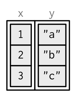
When drawing data frames and tibbles, rather than focusing on the implementation details, i.e. the attributes:

I’ll draw them in the same way as a named list, but arranged to emphasize their columnar structure.
While every element of a data frame (or tibble) must have the same length, both data.frame() and tibble() can recycle shorter inputs. Data frames automatically recycle columns that are an integer multiple of the longest column; tibbles only ever recycle vectors of length 1.
Creating
tibble() is a nice way to create data frames. It encapsulates best practices for data frames:
It never changes an input’s type (i.e., no more stringsAsFactors = FALSE!).
This makes it easier to use with list-columns:
tibble(x = 1:3, y = list(1:5, 1:10, 1:20))
#> # A tibble: 3 x 2
#> x y
#> <int> <list>
#> 1 1 <int [5]>
#> 2 2 <int [10]>
#> 3 3 <int [20]>
List-columns are most commonly created by do(), but they can be useful to create by hand.
It never adjusts the names of variables:
names(data.frame(`crazy name` = 1))
#> [1] "crazy.name"
names(tibble(`crazy name` = 1))
#> [1] "crazy name"
It evaluates its arguments lazily and sequentially:
tibble(x = 1:5, y = x ^ 2)
#> # A tibble: 5 x 2
#> x y
#> <int> <dbl>
#> 1 1 1.00
#> 2 2 4.00
#> 3 3 9.00
#> 4 4 16.0
#> # ... with 1 more row
It never uses row.names(). The whole point of tidy data is to store variables in a consistent way. So it never stores a variable as special attribute.
It only recycles vectors of length 1. This is because recycling vectors of greater lengths is a frequent source of bugs.
Coercion
To complement tibble(), tibble provides as_tibble() to coerce objects into tibbles. Generally, as_tibble() methods are much simpler than as.data.frame() methods, and in fact, it’s precisely what as.data.frame() does, but it’s similar to do.call(cbind, lapply(x, data.frame)) - i.e. it coerces each component to a data frame and then cbinds() them all together.
as_tibble() has been written with an eye for performance:
if (requireNamespace("microbenchmark", quiet = TRUE)) {
l <- replicate(26, sample(100), simplify = FALSE)
names(l) <- letters
microbenchmark::microbenchmark(
as_tibble(l),
as.data.frame(l)
)
}
#> Loading required namespace: microbenchmark
The speed of as.data.frame() is not usually a bottleneck when used interactively, but can be a problem when combining thousands of messy inputs into one tidy data frame.
Tibbles vs data frames
There are three key differences between tibbles and data frames: printing, subsetting, and recycling rules.
Printing
When you print a tibble, it only shows the first ten rows and all the columns that fit on one screen. It also prints an abbreviated description of the column type:
tibble(x = 1:1000)
#> # A tibble: 1,000 x 1
#> x
#> <int>
#> 1 1
#> 2 2
#> 3 3
#> 4 4
#> # ... with 996 more rows
You can control the default appearance with options:
options(tibble.print_max = n, tibble.print_min = m): if there are more than n rows, print only the first m rows. Use options(tibble.print_max = Inf) to always show all rows.
options(tibble.width = Inf) will always print all columns, regardless of the width of the screen.
Subsetting
Tibbles are quite strict about subsetting. [ always returns another tibble. Contrast this with a data frame: sometimes [ returns a data frame and sometimes it just returns a vector:
df1 <- data.frame(x = 1:3, y = 3:1)
class(df1[, 1:2])
#> [1] "data.frame"
class(df1[, 1])
#> [1] "integer"
df2 <- tibble(x = 1:3, y = 3:1)
class(df2[, 1:2])
#> [1] "tbl_df" "tbl" "data.frame"
class(df2[, 1])
#> [1] "tbl_df" "tbl" "data.frame"
To extract a single column use [[ or $:
class(df2[[1]])
#> [1] "integer"
class(df2$x)
#> [1] "integer"
Tibbles are also stricter with $. Tibbles never do partial matching, and will throw a warning and return NULL if the column does not exist:
df <- data.frame(abc = 1)
df$a
#> [1] 1
df2 <- tibble(abc = 1)
df2$a
#> Warning: Unknown or uninitialised column: 'a'.
#> NULL
As of version 1.4.1, tibbles no longer ignore the drop argument:
data.frame(a = 1:3)[, "a", drop = TRUE]
#> [1] 1 2 3
tibble(a = 1:3)[, "a", drop = TRUE]
#> [1] 1 2 3
Recycling
When constructing a tibble, only values of length 1 are recycled. The first column with length different to one determines the number of rows in the tibble, conflicts lead to an error. This also extends to tibbles with zero rows, which is sometimes important for programming:
tibble(a = 1, b = 1:3)
#> # A tibble: 3 x 2
#> a b
#> <dbl> <int>
#> 1 1.00 1
#> 2 1.00 2
#> 3 1.00 3
tibble(a = 1:3, b = 1)
#> # A tibble: 3 x 2
#> a b
#> <int> <dbl>
#> 1 1 1.00
#> 2 2 1.00
#> 3 3 1.00
tibble(a = 1:3, c = 1:2)
#> Error: Column `c` must be length 1 or 3, not 2
tibble(a = 1, b = integer())
#> # A tibble: 0 x 2
#> # ... with 2 variables: a <dbl>, b <int>
tibble(a = integer(), b = 1)
#> # A tibble: 0 x 2
#> # ... with 2 variables: a <int>, b <dbl>