Chapter 1.2.5.2 Sampling Distributions

We describe $t$ , $χ2$ and $F$ in the context of samples from normal rv.

Emphasis is on understanding relationship between the rv and how it comes about from $X¯$ and $S$ .

The goal is for you not to be surprised when we say later that test statistics have certain distributions. You may not be able to prove it, but hopefully won’t be surprised either. We’ll use density estimation extensively to illustrate the relationships.

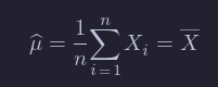
Given $X1,\dots,Xn$ , which we assume in this section are independent and identically distributed with mean $μ$ and standard deviation $σ$ , we define the sample mean

X¯ = \sumi=1n Xi

and the sample standard deviation

S^2 = 1/(n-1) \sumi=1n (Xi-X¯)^2

We note that $X¯$ is an estimator for $μ$ and $S$ is an estimator for $σ$ .

Summary

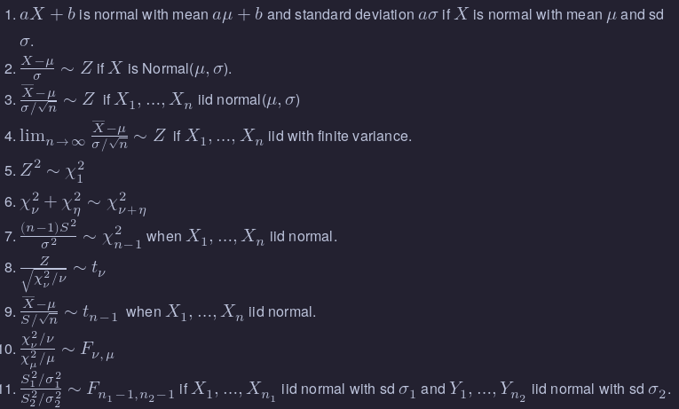
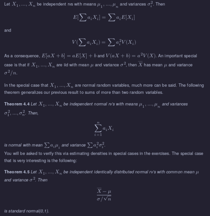
Linear Combination of Normal RVs

Point Estimators

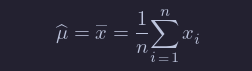
If $X$ is a random variable that depends on parameter $β$ , then often we are interested in estimating the value of $β$ from a random sample $X1,\dots,Xn$ from $X$ . For example, if $X$ is a normal rv with unknown mean $μ$ , and we get data $X1,\dots,Xn$ , it would be very natural to estimate $μ$ by $1/n\sumi=1nXi.$

Notationally, we say

In other words, our estimate of $β$ from the data $x1,\dots,xn$ is denoted by $β^$ .

The two point estimators that we are interested in at this point are point estimators for the $mean$ of an rv and the $variance$ of an rv. (Note that we have switched gears a little bit, because the mean and variance aren’t necessarily parameters of the rv. We are really estimating functions of the parameters at this point. The distinction will not be important for the purposes of this text.) Recall that the definition of the mean of a discrete rv with possible values $xi$ is

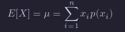
If we are given data $x1,\dots,xn$ , it is natural to assign $p(xi)=1/n$ for each of those data points to create a new random variable $X0$ , and we obtain

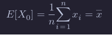
This is a natural choice for our point estimator for the mean of the rv $X$ , as well.

Continuing in the same way, if we are given data $x1,\dots,xn$ and we wish to estimate the variance, then we could create a new random variable $X0$ whose possible outcomes are $x1,\dots,xn$ with probabilities $1/n$ , and compute

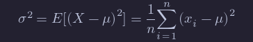
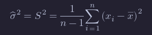
This works just fine as long as $μ$ is known. However, most of the time, we do not know $μ$ and we must replace the true value of $μ$ with our estimate from the data.

There is a heuristic that each time you replace a parameter with an estimate of that parameter, you divide by one less. Following that heuristic, we obtain

Properties of Point Estimators

Note that the point estimators for $μ$ and $σ^2$ can be thought of as random variables themselves, since they are combinations of a random sample from a distribution. As such, they also have distributions, means and variances.

One property of point estimators that is often desirable is that it is unbiased. We say that a point estimator $β^$ for $β$ is unbiased if $E[β^]=β$ . (Recall: $β^$ is a random variable, so we can take its expected value!) Intuitively, unbiased means that the estimator does not consistently underestimate or overestimate the parameter it is estimating. If were to estimate the parameter over and over again, the average value would converge to the correct value of the parameter.

Let’s consider $x¯$ and $S^2$ . Are they unbiased? It is possible to determine this analytically, and interested students should consult Wackerly et al for a proof. However, we will do this using R and simulation.

Variance of Unbiased Estimators

From the above, we can see that $x¯$ and $S^2$ are unbiased estimators for $μ$ and $σ^2$ , respectively. There are other unbiased estimator for the mean and variance, however.

For example, if $X1,\dots,Xn$ is a random sample from a normal rv, then the median of the $X i is also an unbiased estimator for the mean$ . Moreover, the median seems like a perfectly reasonable thing to use to estimate $μ$ , and in many cases is actually preferred to the mean.

There is one way, however, in which the sample mean $x¯$ is definitely better than the median, and that is that it has a lower variance. So, in theory at least, $x¯$ should not deviate from the true mean as much as the median will deviate from the true mean, as measured by variance.

Sample Variance

In many practical situations, the true variance of a population is not known a priori and must be computed somehow. When dealing with extremely large populations, it is not possible to count every object in the population, so the computation must be performed on a sample of the population.^[8] Sample variance can also be applied to the estimation of the variance of a continuous distribution from a sample of that distribution.

We take a sample with replacement of n values y₁, ..., y_n from the population, where n < N, and estimate the variance on the basis of this sample.^[9] Directly taking the variance of the sample data gives the average of the squared deviations:

\sigma _{y}^{2}={\frac {1}{n}}\sum _{i=1}^{n}\left(y_{i}-{\overline {y}}\right)^{2}=\left({\frac {1}{n}}\sum _{i=1}^{n}y_{i}^{2}\right)-{\overline {y}}^{2}={\frac {1}{n^{2}}}\sum _{i<j}\left(y_{i}-y_{j}\right)^{2}.

Here, ${\overline {y}}$ denotes the sample mean:

{\overline {y}}={\frac {1}{n}}\sum _{i=1}^{n}y_{i}.

Since the y_i are selected randomly, both ${\overline {y}}$ and $\sigma _{y}^{2}$ are random variables. Their expected values can be evaluated by averaging over the ensemble of all possible samples {y_i} of size n from the population. For $\sigma _{y}^{2}$ this gives:

{\begin{aligned}\operatorname {E} [\sigma _{y}^{2}]&=\operatorname {E} \left[{\frac {1}{n}}\sum _{i=1}^{n}\left(y_{i}-{\frac {1}{n}}\sum _{j=1}^{n}y_{j}\right)^{2}\right]\\&={\frac {1}{n}}\sum _{i=1}^{n}\operatorname {E} \left[y_{i}^{2}-{\frac {2}{n}}y_{i}\sum _{j=1}^{n}y_{j}+{\frac {1}{n^{2}}}\sum _{j=1}^{n}y_{j}\sum _{k=1}^{n}y_{k}\right]\\&={\frac {1}{n}}\sum _{i=1}^{n}\left[{\frac {n-2}{n}}\operatorname {E} [y_{i}^{2}]-{\frac {2}{n}}\sum _{j\neq i}\operatorname {E} [y_{i}y_{j}]+{\frac {1}{n^{2}}}\sum _{j=1}^{n}\sum _{k\neq j}^{n}\operatorname {E} [y_{j}y_{k}]+{\frac {1}{n^{2}}}\sum _{j=1}^{n}\operatorname {E} [y_{j}^{2}]\right]\\&={\frac {1}{n}}\sum _{i=1}^{n}\left[{\frac {n-2}{n}}(\sigma ^{2}+\mu ^{2})-{\frac {2}{n}}(n-1)\mu ^{2}+{\frac {1}{n^{2}}}n(n-1)\mu ^{2}+{\frac {1}{n}}(\sigma ^{2}+\mu ^{2})\right]\\&={\frac {n-1}{n}}\sigma ^{2}.\end{aligned}}

Hence $\sigma _{y}^{2}$ gives an estimate of the population variance that is biased by a factor of ${\frac {n-1}{n}}$ . For this reason, $\sigma _{y}^{2}$ is referred to as the biased sample variance. Correcting for this bias yields the unbiased sample variance:

s^{2}={\frac {n}{n-1}}\sigma _{y}^{2}={\frac {n}{n-1}}\left({\frac {1}{n}}\sum _{i=1}^{n}\left(y_{i}-{\overline {y}}\right)^{2}\right)={\frac {1}{n-1}}\sum _{i=1}^{n}\left(y_{i}-{\overline {y}}\right)^{2}

Either estimator may be simply referred to as the sample variance when the version can be determined by context. The same proof is also applicable for samples taken from a continuous probability distribution.

The use of the term n − 1 is called Bessel's correction, and it is also used in sample covariance and the sample standard deviation (the square root of variance). The square root is a concave function and thus introduces negative bias (by Jensen's inequality), which depends on the distribution, and thus the corrected sample standard deviation (using Bessel's correction) is biased. The unbiased estimation of standard deviation is a technically involved problem, though for the normal distribution using the term n − 1.5 yields an almost unbiased estimator.

The unbiased sample variance is a U-statistic for the function ƒ(y₁, y₂) = (y₁ − y₂)²/2, meaning that it is obtained by averaging a 2-sample statistic over 2-element subsets of the population.

Distribution of the sample variance

Distribution and cumulative distribution of s²/σ², for various values of ν = n − 1, when the y_i are independent normally distributed.

Being a function of random variables, the sample variance is itself a random variable, and it is natural to study its distribution. In the case that y_i are independent observations from a normal distribution, Cochran's theorem shows that s² follows a scaled chi-squared distribution:^[10]

(n-1){\frac {s^{2}}{\sigma ^{2}}}\sim \chi _{n-1}^{2}.

As a direct consequence, it follows that

\operatorname {E} (s^{2})=\operatorname {E} \left({\frac {\sigma ^{2}}{n-1}}\chi _{n-1}^{2}\right)=\sigma ^{2},

and^[11]

\operatorname {Var} [s^{2}]=\operatorname {Var} \left({\frac {\sigma ^{2}}{n-1}}\chi _{n-1}^{2}\right)={\frac {\sigma ^{4}}{(n-1)^{2}}}\operatorname {Var} \left(\chi _{n-1}^{2}\right)={\frac {2\sigma ^{4}}{n-1}}.

If the y_i are independent and identically distributed, but not necessarily normally distributed, then^[12]^[13]

\operatorname {E} [s^{2}]=\sigma ^{2},\quad \operatorname {Var} [s^{2}]={\frac {\sigma ^{4}}{n}}\left((\kappa -1)+{\frac {2}{n-1}}\right)={\frac {1}{n}}\left(\mu _{4}-{\frac {n-3}{n-1}}\sigma ^{4}\right),

where κ is the kurtosis of the distribution and μ₄ is the fourth central moment.

If the conditions of the law of large numbers hold for the squared observations, s² is a consistent estimator of σ². One can see indeed that the variance of the estimator tends asymptotically to zero. An asymptotically equivalent formula was given in Kenney and Keeping (1951:164), Rose and Smith (2002:264), and Weisstein (n.d.).^[14]^[15]^[16]

Chi-squared

Let $Z$ be a standard normal(0,1) random variable.

An rv with the same distribution $Z^2$ is called a Chi-squared rv with one degree of freedom. The sum of $n$ independent $χ2$ rv’s with 1 degree of freedom is a chi-squared rv with $n$ degrees of freedom.

In particular, the sum of a $χ2$ with $ν1$ degrees of freedom and a $χ2$ with $ν2$ degrees of freedom is $χ2$ with $ν1+ν2$ degrees of freedom.

sdData <- replicate(10000, 3/81 * sd(rnorm(4, 3, 9))^2)
f <- function(x) dchisq(x, df = 3)
ggplot(data.frame(sdData), aes(x = sdData)) + 
  geom_density() +
  stat_function(fun = f, color = "red")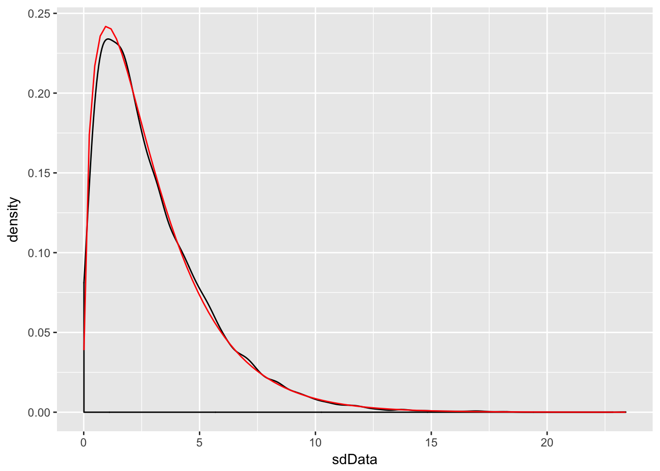

Theorem

Let

X1,\dots,Xn

be iid normal random variables. Then,

(n-1/σ^2)*S^2

has a

χ2

distribution with

n-1

degrees of freedom.

F distribution

An $F$ distribution has the same density function as

Fν1,ν2=χν1^2/ν1 / χν2^2/ν2

We say $F$ has $ν1$ numerator degrees of freedom and $ν2$ denominator degrees of freedom.

One example of this type is:

S1^2/σ1^2 / S2^2/σ2^2

where $X1,\dots,Xn1$ are iid normal with standard deviation $σ1$

and $Y1,\dots,Yn2$ are iid normal with standard deviation $σ2.$

$t$ distribution

If $Z$ is a standard normal(0,1) rv, $χν2$ is a Chi-squared rv with $ν$ degrees of freedom, and $Z$ and $χν2$ are independent, then

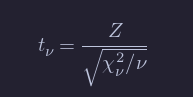
is distributed as a $t$ random variable with $ν$ degrees of freedom.

Theorem

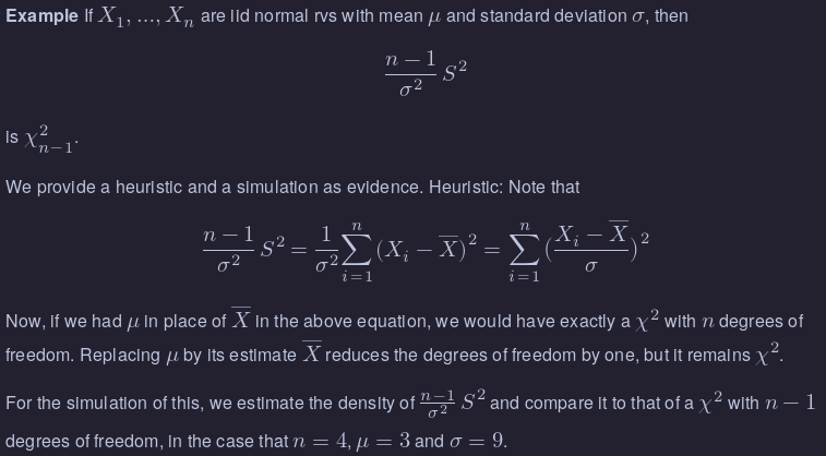
If $X1,\dots,Xn$ are iid normal rvs with mean $μ$ and sd $σ$ , then

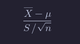
is $t$ with $n-1$ degrees of freedom.

Note that $X¯-μ/ σ/sqrt{n}$ is normal(0,1). So, replacing $σ$ with $S$ changes the distribution from normal to $t$ .

R as a set of statistical tables

One convenient use of R is to provide a comprehensive set of statistical tables.

Functions are provided to evaluate the cumulative distribution function P(X <= x), the probability density function and the quantile function (given q, the smallest x such that P(X <= x) > q), and to simulate from the distribution.

Distribution R name additional arguments

beta beta shape1, shape2, ncp

binomial binom size, prob

Cauchy cauchy location, scale

chi-squared chisq df, ncp

exponential exp rate

F f df1, df2, ncp

gamma gamma shape, scale

geometric geom prob

hypergeometric hyper m, n, k

log-normal lnorm meanlog, sdlog

logistic logis location, scale

negative binomial nbinom size, prob

normal norm mean, sd

Poisson pois lambda

signed rank signrank n

Student’s t t df, ncp

uniform unif min, max

Weibull weibull shape, scale

Wilcoxon wilcox

Distribution	R name	additional arguments
beta	`beta`	`shape1, shape2, ncp`
binomial	`binom`	`size, prob`
Cauchy	`cauchy`	`location, scale`
chi-squared	`chisq`	`df, ncp`
exponential	`exp`	`rate`
F	`f`	`df1, df2, ncp`
gamma	`gamma`	`shape, scale`
geometric	`geom`	`prob`
hypergeometric	`hyper`	`m, n, k`
log-normal	`lnorm`	`meanlog, sdlog`
logistic	`logis`	`location, scale`
negative binomial	`nbinom`	`size, prob`
normal	`norm`	`mean, sd`
Poisson	`pois`	`lambda`
signed rank	`signrank`	`n`
Student’s t	`t`	`df, ncp`
uniform	`unif`	`min, max`
Weibull	`weibull`	`shape, scale`
Wilcoxon	`wilcox`

Prefix the name given here by ‘d’ for the density, ‘p’ for the CDF, ‘q’ for the quantile function and ‘r’ for simulation (random deviates). The first argument is x for dxxx, q for pxxx, p for qxxx and n for rxxx (except for rhyper, rsignrank and rwilcox, for which it is nn). In not quite all cases is the non-centrality parameter ncp currently available: see the on-line help for details.

The pxxx and qxxx functi overridden.ons all have logical arguments lower.tail and log.p and the dxxx ones have log. This allows, e.g., getting the cumulative (or “integrated”) hazard function, H(t) = - log(1 - F(t)), by
 - pxxx(t, ..., lower.tail = FALSE, log.p = TRUE)
or more accurate log-likelihoods (by dxxx(..., log = TRUE)), directly.

In addition there are functions ptukey and qtukey for the distribution of the studentized range of samples from a normal distribution, and dmultinom and rmultinom for the multinomial distribution. Further distributions are available in contributed packages, notably SuppDists.

See the on-line help on RNG for how random-number generation is done in R.