Chapter 1.2.1 Special Discrete Random Variables

In the below sections, we discuss the binomial, geometric and poisson random variables, and their implementation in R.

In order to understand the binomial and geometric rv’s, we will consider the notion of Bernoulli trials.

A Bernoulli trial is an experiment that can result in two outcomes, which we will denote as “Success” and “Failure”. The probability of a success will be denoted p. A typical example would be tossing a coin and considering heads to be a success, where p=.5.

Binomial Random Variable

Several random variables consist of repeated independent Bernoulli trials, with common probability of success p.

Definition

The binomial random variable counts the number of successes observed when n independent Bernoulli trials are formed, each of which has probability of success p.

If X is binomial with number of trials n and probability of success p, then

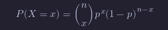
Here, P(X = x) is the probability that we observe x successes. Note that

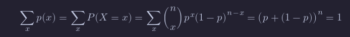
by the binomial expansion theorem.

Example

+Suppose 100 dice are thrown. What is the probability of observing 10 or fewer sixes? We assume that the results of the dice are independent and that the probability of rolling a six is p = 1/6.

Then, the probability of observing 10 or fewer sixes is

P(X≤10) = ∑j=0 10 P(X=j)

where X is binomial with parameters n=100 and p = 1/6.

The R command for computing this is sum(dbinom(0:10, 100, 1/6))

or pbinom(10,100,1/6).

We will discuss in detail the various *binom commands in Section 3.7.

Theorem

Let X be a binomial random variable with n trials and probability of success p. Then

• The expected value of X is np.
• The variance of X is np(1−p).

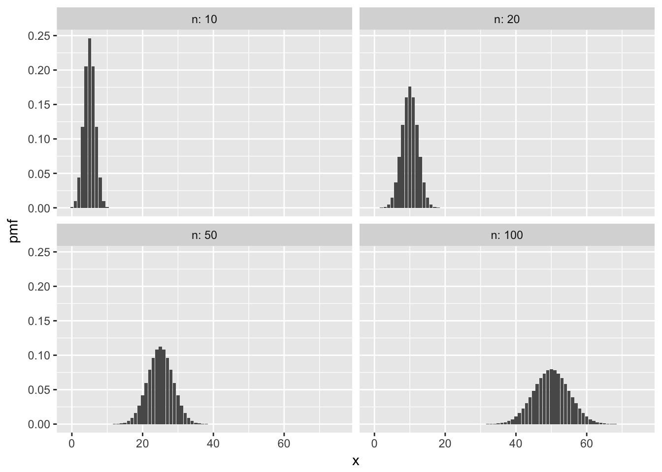
Here are some sample plots of the pmf of a binomial rv for various values of n and p=.5².

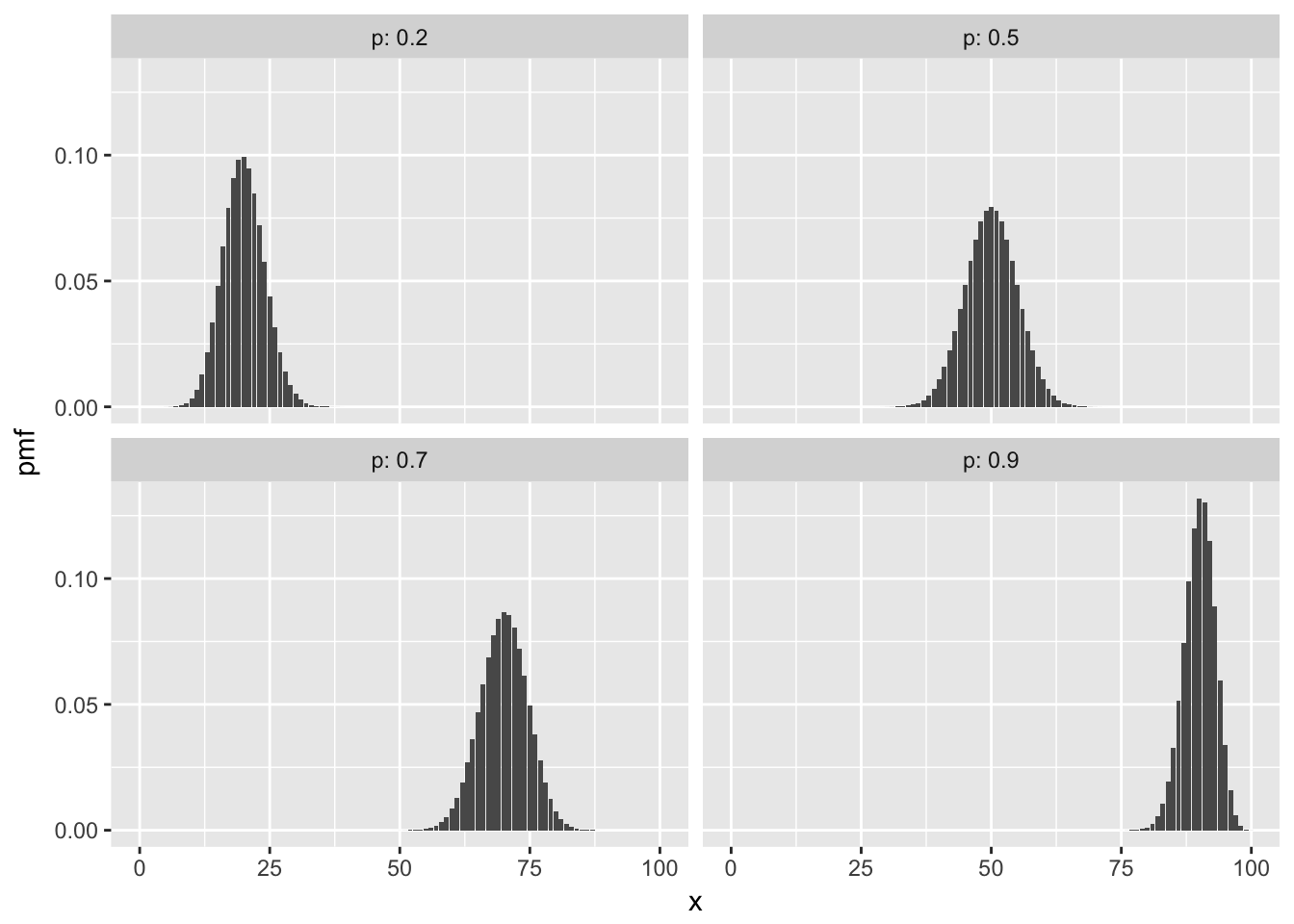
Here are some with n = 100 and various p.

Negative Binomial Random Variable

Example

Suppose you repeatedly roll a fair die. What is the probability of getting exactly 14 non-sixes before getting your second 6?

As you can see, this is an example of repeated Bernoulli trials with p= 1/6, but it isn’t exactly geometric because we are waiting for the second success. This is an example of a negative binomial random variable.

More generally, suppose that we observe a sequence of Bernoulli trials with probability of success prob. If X denotes the number of failures x before the nth success, then X is a negative binomial random variable with parameters n and p. The probability mass function of X is given by

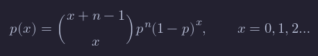
The mean of a negative binomial is np/(1−p), and the variance is np/(1−p)2.

The root R function to use with negative binomials is nbinom, so dnbinom is how we can compute values in R.

The function dnbinom uses prob for p and size for n in our formula. So, to continue with the example above, the probability of obtaining exactly 14 non-sixes before obtaining 2 sixes is:

dnbinom(x = 14, size = 2, prob = 1/6)

## [1] 0.03245274

Geometric Random Variable

Definition

A geometric random variable counts the number of failures in Bernoulli trials until the first success occurs.

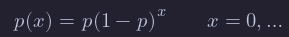
A geometric random variable can take on values 0,1,2,…

The pmf of a geometric rv is given by

Note that

∑ xp(x) = 1

by the sum of a geometric series formula.

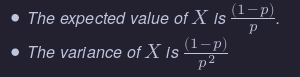
Theorem

Let X be a geometric random variable with probability of success p. Then

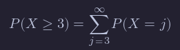
Example A die is tossed until the first 6 occurs. What is the probability that it takes 4 or more tosses? We let X be a geometric random variable with probability of success 1/6. Since X counts the number of failures before the first success, the problem is asking us to compute

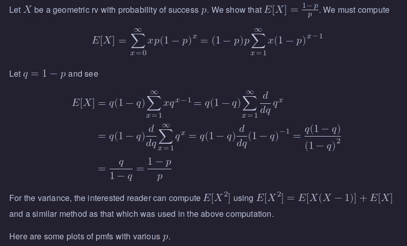
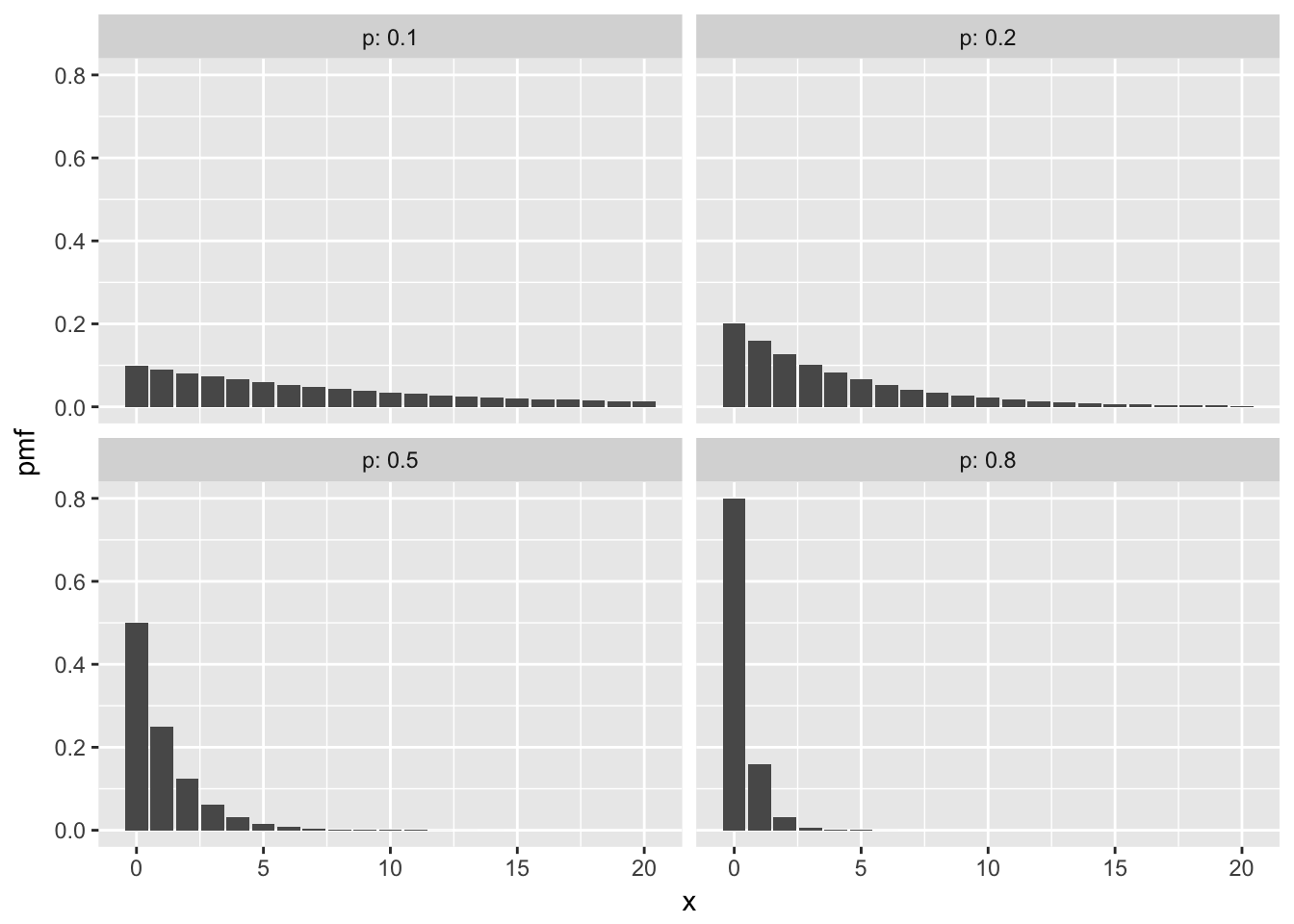
Proof that the mean of a geometric rv is 1−p/p(Optional)