Chapter 6.1.1 Hypothesis Testing

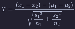
Suppose that you have null hypothesis $H_0:p=p_0$and alternative $H_a:p\ne p_0$. You run $n$ trials and obtain $x$ successes, so your estimate for $p$ is given by $\hat{p}=x/n$. Presumably, $\hat{p}$ is not exactly equal to $p_0$, and you wish to determine the probability of obtaining an estimate that far away from $p_0$ or further.

Formally, we are going to add the probabilities of all outcomes that are no more likely than the outcome that was obtained, since if we are going to reject when we obtain $x$successes, we would also reject if we obtain a number of successes that was even less likely to occur.

Example

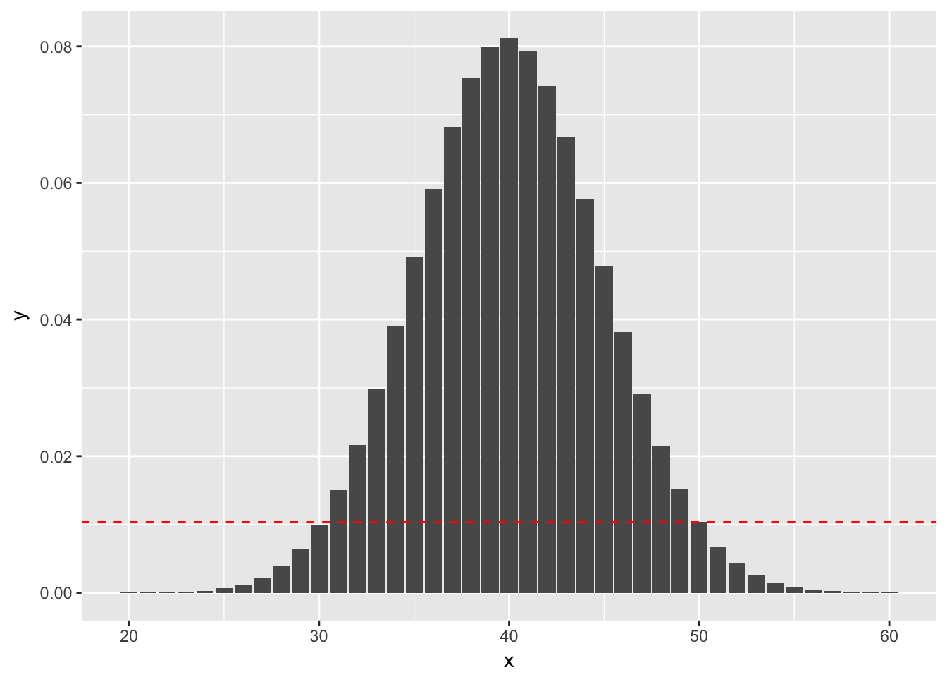
(Using binom.test) Suppose you wish to test $H_0:p=0.4$versus $H_a:p\ne 0.4$. You do 100 trials and obtain 50 successes.The probability of getting exactly 50 successes is dbinom(50, 100, 0.4), or 0.01034. Anything more than 50 successes is less likely under the null hypothesis, so we would add all of those to get part of our $p$-value. To determine which values we add for successes less than 50 we look for all outcomes that have probability of occurring (under the null hypothesis) less than 0.01034. Namely, those are the outcomes between 0 and 30, since dbinom(30, 100, 0.4) is 0.1001. See also the following figure, where the dashed red line indicates the likelihood of observing exactly 50 successes. We sum all of the probabilities that are below the dashed red line. (Note that the x-axis has been truncated.)

So, the $p$-value would be $$P(X\le 30)+P(X\ge 50)$$

where $X\sim$ Binomial(n = 100, p = 0.4).

Example

(Using prop.test)

When $n$ is large and $p$ isn’t too close to 0 or 1, binomial random variables with $n$ trials and probability of success $p$ can be approximated by normal random variables with mean $np$ and standard deviation $\sqrt{np(1-p)}$. This can be used to get approximate $p$-values associated with the hypothesis test $H_0:p=p_0$ versus $H_a:p\ne p_0$.

We consider again the example that in 100 trials, you obtain 50 successes when testing $H_0:p=0.4$versus $H_a:p\ne 0.4$. Let $X$ be a binomial random variable with $n=100$ and $p=0.4$.

We approximate $X$ by a normal rv $N$ with mean $np=40$ and standard deviation $\sqrt{np(1-p)}=4.89879$. As before, we need to compute the probability under $H_0$ of obtaining an outcome that is as likely or less likely than obtaining 50 successes. However, in this case, we are using the normal approximation, which is symmetric about its mean. Therefore, the $p$-value would be $$P(N\ge 50)+P(N\le 30)$$

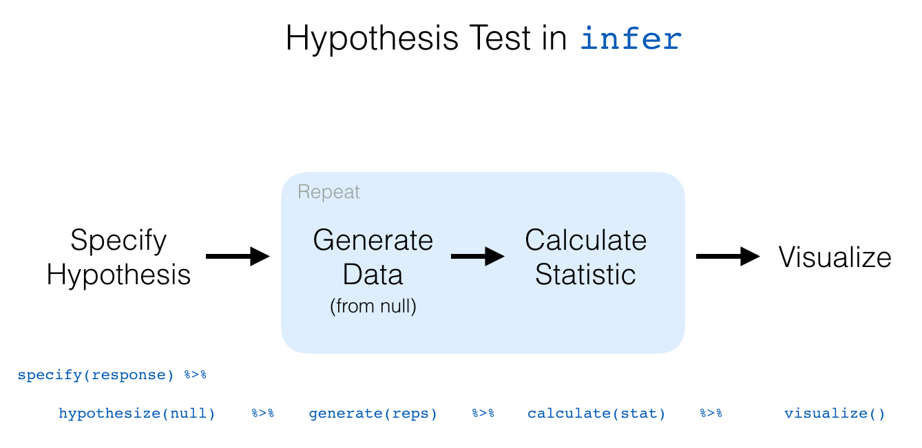
Hypothesis testing with infer

The “There is Only One Test” diagram mentioned in Section 10.2 was the inspiration for the infer pipeline that you saw for confidence intervals in Chapter 9. For hypothesis tests, we include one more verb into the pipeline: the hypothesize() verb. Its main argument is null which is either

• "point" for point hypotheses involving a single sample or
• "independence" for testing for independence between two variables.

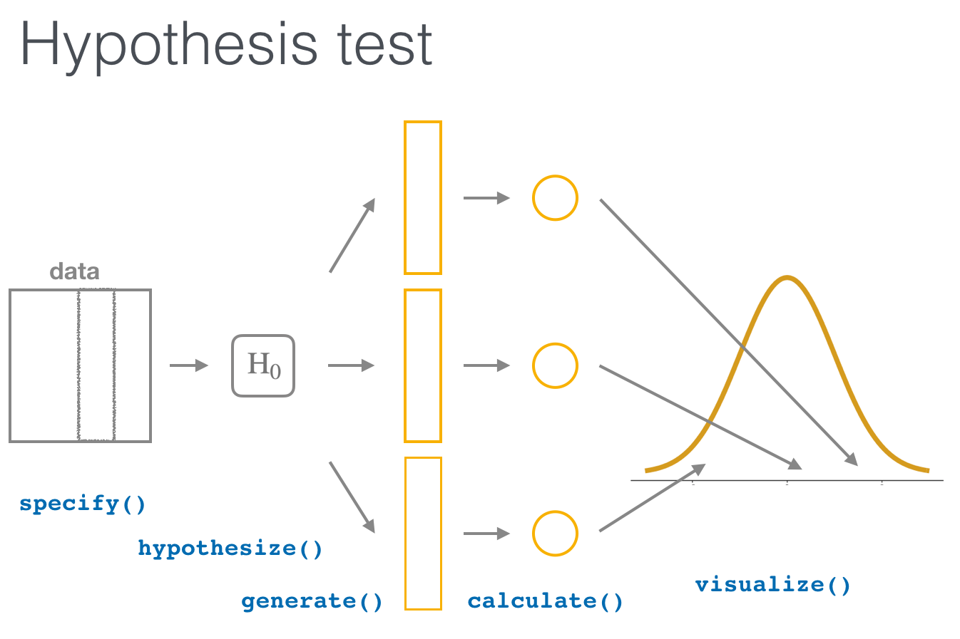
We’ll first explore the two variable case by comparing two means. Note the section headings here that refer to the “There is Only One Test” diagram. We will lay out the specifics for each problem using this framework and the infer pipeline together.

We conclude by showing the infer pipeline diagram. In Chapter 11, we’ll come back to regression and see how the ideas covered in Chapter 9 and this chapter can help in understanding the significance of predictors in modeling.

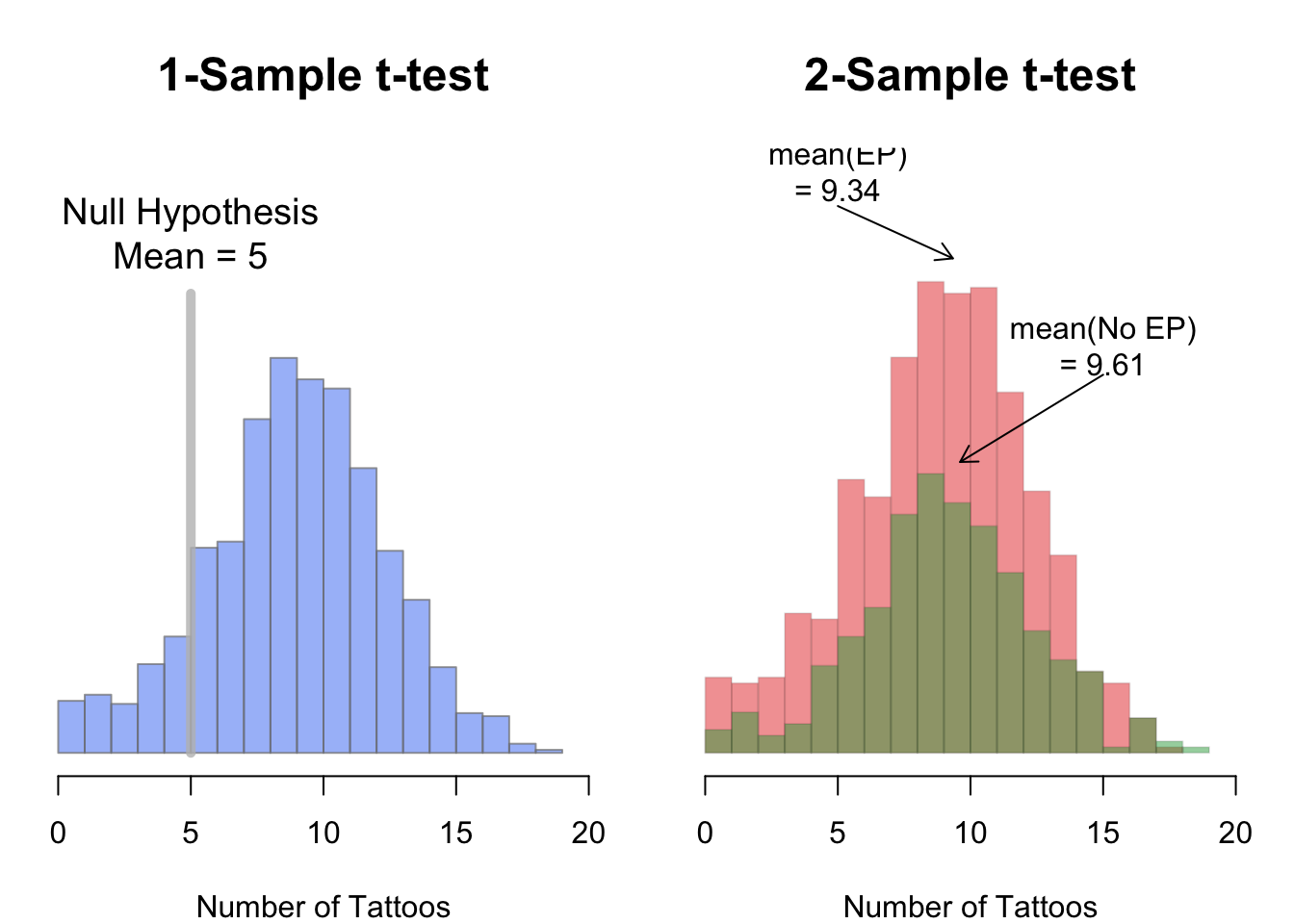
Two sample hypothesis tests of ${\mu }_1={\mu }_2$

Here, we present a couple of examples of two sample t tests. In this situation, we have two populations that we are sampling from, and we are wondering whether the mean of population one differs from the mean of population two. At least, that is the problem we are typically working on!

The assumptions for t tests remain the same. We are assuming that the underlying populations are normal, or that we have enough samples so that the central limit theorem takes hold. We are also AS ALWAYS assuming that there are no outliers. Remember: outliers can kill t tests. Both the one-sample and the two-sample variety.

We also have two other choices.

1. We can assume that the variances of the two populations are equal. If the variances of the two populations really are equal, then this is the correct thing to do. In general, it is a more conservative approach not to assume the variances of the two populations are equal, and I generally recommend not to assume equal variance unless you have a good reason for doing so.
2. Whether the data is paired or unpaired. Paired data results from multiple measurements of the same individual at different times, while unpaired data results from measurements of different individuals. Say, for example, you wish to determine whether a new fertilizer increases the mean number of apples that apple trees produce. If you count the number of apples one season, and then the next season apply the fertilizer and count the number of apples again, then you would expect there to be some relationship between the number of apples you count in each season (big trees would have more apples each season than small trees, for example). If you randomly selected half of the trees to apply fertilizer to in one growing season, then there would not be any dependencies in the data. In general, it is a hard problem to deal with dependent data, but paired data is one type of data that we can deal with.

Example

Consider the data in anorexia in the MASS library. Is there sufficient evidence to conclude that there is a difference in the pre- and post- treatment weights of girls receiving the CBT treatment?

Formally, we let ${\mu }_1$denote the mean pre-treatment weight of girls with anorexia, and we let ${\mu }_2$ denote the mean post-CBT treatment weight of girls with anorexia. We test $$H_0:{\mu }_1={\mu }_2$$ versus $$H_a:{\mu }_1<{\mu }_2$$

We choose a one-sided test because we have reason to believe that the CBT treatment will help the girls gain weight, and I am doing so before looking at the data. I will not reject the null hypothesis if it turns out that the post treatment weight is less than the pre treatment weight.

Additionally, since we are doing repeated measurements on the same individuals, this data is paired and dependent. We will need to include paired = TRUE when we call t.test.

The assumptions of t tests are: the pre and post treatment weights are normally distributed (we can do less than that in this case, since we have paired data, but…), or that the population is close enough to normal for the sample size that we have, and that the weights are independent (except for being paired). I am willing to make those assumptions for this experiment. The data is plotted below; please take a look at the plots.

Comparing two means

1. Randomization/permutation

We will now focus on building hypotheses looking at the difference between two population means in an example. We will denote population means using the Greek symbol $\mu$(pronounced “mu”). Thus, we will be looking to see if one group “out-performs” another group. This is quite possibly the most common type of statistical inference and serves as a basis for many other types of analyses when comparing the relationship between two variables.

Our null hypothesis will be of the form $H_0:{\mu }_1={\mu }_2$, which can also be written as $H_0:{\mu }_1-{\mu }_2=0$. Our alternative hypothesis will be of the form $H_0:{\mu }_1\star {\mu }_2$ (or $H_a:{\mu }_1-{\mu }_2\star 0$) where $\star$ = $<$, $\ne$, or $>$depending on the context of the problem. You needn’t focus on these new symbols too much at this point. It will just be a shortcut way for us to describe our hypotheses.

As we saw in Chapter 9, bootstrapping is a valuable tool when conducting inferences based on one or two population variables. We will see that the process of randomization (also known as permutation) will be valuable in conducting tests comparing quantitative values from two groups.

Important note: Remember that we hardly ever have access to the population values as we do here. This example and the nycflights13 dataset were used to create a common flow from chapter to chapter. In nearly all circumstances, we’ll be needing to use only a sample of the population to try to infer conclusions about the unknown population parameter values. These examples do show a nice relationship between statistics (where data is usually small and more focused on experimental settings) and data science (where data is frequently large and collected without experimental conditions).

2. Sampling $\to$randomization

We can use hypothesis testing to investigate ways to determine, for example, whether a treatment has an effect over a control and other ways to statistically analyze if one group performs better than, worse than, or different than another. We are interested here in seeing how we can use a random sample of action movies and a random sample of romance movies from movies to determine if a statistical difference exists in the mean ratings of each group.

3. Data

Do we have reason to believe, based on the sample distributions of rating over the two groups of genre, that there is a significant difference between the mean rating for action movies compared to romance movies? It’s hard to say just based on the plots. The boxplot does show that the median sample rating is higher for romance movies, but the histogram isn’t as clear. The two groups have somewhat differently shaped distributions but they are both over similar values of rating. It’s often useful to calculate the mean and standard deviation as well, conditioned on the two levels.

4. Model of $H_0$

The hypotheses we specified can also be written in another form to better give us an idea of what we will be simulating to create our null distribution.

• $H_0:{\mu }_r-{\mu }_a=0$

• $H_a:{\mu }_r-{\mu }_a\ne 0$

5. Test statistic $\delta$

We are, therefore, interested in seeing whether the difference in the sample means, ${\overline{x}}_r-{\overline{x}}_a$, is statistically different than 0. We can now come back to our infer pipeline for computing our observed statistic. Note the order argument that shows the mean value for "Action" being subtracted from the mean value of "Romance".

6. Simulated data

Tactile simulation

Here, with us assuming the two population means are equal ($H_0:{\mu }_r-{\mu }_a=0$), we can look at this from a tactile point of view by using index cards. There are $n_r=34$ data elements corresponding to romance movies and $n_a=34$for action movies. We can write the 34 ratings from our sample for romance movies on one set of 34 index cards and the 34 ratings for action movies on another set of 34 index cards. (Note that the sample sizes need not be the same.)

The next step is to put the two stacks of index cards together, creating a new set of 68 cards. If we assume that the two population means are equal, we are saying that there is no association between ratings and genre (romance vs action). We can use the index cards to create two new stacks for romance and action movies. First, we must shuffle all the cards thoroughly. After doing so, in this case with equal values of sample sizes, we split the deck in half.

We then calculate the new sample mean rating of the romance deck, and also the new sample mean rating of the action deck. This creates one simulation of the samples that were collected originally. We next want to calculate a statistic from these two samples. Instead of actually doing the calculation using index cards, we can use R as we have before to simulate this process. Let’s do this just once and compare the results to what we see in movies_genre_sample.

7. Distribution of $\delta$under $H_0$

The generate() step completes a permutation sending values of ratings to potentially different values of genre from which they originally came.

It simulates a shuffling of the ratings between the two levels of genre just as we could have done with index cards. We can now proceed in a similar way to what we have done previously with bootstrapping by repeating this process many times to create simulated samples, assuming the null hypothesis is true.

Hypothesis Tests

Chi-square: chsq.test()

Next, we’ll cover chi-square tests. In a chi-square test test, we test whether or not there is a difference in the rates of outcomes on a nominal scale (like sex, eye color, first name etc.). The test statistic of a chi-square text is ${\chi }^2$ and can range from 0 to Infinity. The null-hypothesis of a chi-square test is that ${\chi }^2$ = 0 which means no relationship.

A key difference between the chisq.test() and the other hypothesis tests we’ve covered is that chisq.test() requires a table created using the table() function as its main argument. You’ll see how this works when we get to the examples.

1-sample Chi-square test

If you conduct a 1-sample chi-square test, you are testing if there is a difference in the number of members of each category in the vector. Or in other words, are all category memberships equally prevalent? Here’s the general form of a one-sample chi-square test:

# General form of a one-sample chi-square test
chisq.test(x = table(x))

As you can see, the main argument to chisq.test() should be a table of values created using the table() function. For example, let’s conduct a chi-square test to see if all pirate colleges are equally prevalent in the pirates data. We’ll start by creating a table of the college data:

# Frequency table of pirate colleges
table(pirates$college)
##  CCCC JSSFP 
##   658   342

Just by looking at the table, it looks like pirates are much more likely to come from Captain Chunk’s Cannon Crew (CCCC) than Jack Sparrow’s School of Fashion and Piratery (JSSFP). For this reason, we should expect a very large test statistic and a very small p-value. Let’s test it using the chisq.test() function.

# Are all colleges equally prevelant?
college.cstest <- chisq.test(x = table(pirates$college))
college.cstest
##  Chi-squared test for given probabilities
## data:  table(pirates$college)
## X-squared = 100, df = 1, p-value <2e-16

Indeed, with a test statistic of 99.86 and a tiny p-value, we can safely reject the null hypothesis and conclude that certain college are more popular than others.

2-sample Chi-square test

If you want to see if the frequency of one nominal variable depends on a second nominal variable, you’d conduct a 2-sample chi-square test. For example, we might want to know if there is a relationship between the college a pirate went to, and whether or not he/she wears an eyepatch. We can get a contingency table of the data from the pirates dataframe as follows:

# Do pirates that wear eyepatches have come from different colleges
#  than those that do not wear eyepatches?
table(pirates$eyepatch, 
      pirates$college)
##     CCCC JSSFP
##   0  225   117
##   1  433   225

To conduct a chi-square test on these data, we will enter table of the two data vectors:

# Is there a relationship between a pirate's
# college and whether or not they wear an eyepatch?

colpatch.cstest <- chisq.test(x = table(pirates$college,
                                        pirates$eyepatch))
colpatch.cstest
##  Pearson's Chi-squared test with Yates' continuity correction
## data:  table(pirates$college, pirates$eyepatch)
## X-squared = 0, df = 1, p-value = 1

It looks like we got a test statistic of ${\chi }^2$= 0 and a p-value of 1. At the traditional p = .05 threshold for significance, we would conclude that we fail to reject the null hypothesis and state that we do not have enough information to determine if pirates from different colleges differ in how likely they are to wear eye patches.

Getting APA-style conclusions with the apa function

Most people think that R pirates are a completely unhinged, drunken bunch of pillaging buffoons. But nothing could be further from the truth! R pirates are a very organized and formal people who like their statistical output to follow strict rules. The most famous rules are those written by the American Pirate Association (APA). These rules specify exactly how an R pirate should report the results of the most common hypothesis tests to her fellow pirates.

For example, in reporting a t-test, APA style dictates that the result should be in the form t(df) = X, p = Y (Z-tailed), where df is the degrees of freedom of the text, X is the test statistic, Y is the p-value, and Z is the number of tails in the test. Now you can of course read these values directly from the test result, but if you want to save some time and get the APA style conclusion quickly, just use the apa function.

t.test()

To compare the mean of 1 group to a specific value, or to compare the means of 2 groups, you do a t-test. The t-test function in R is t.test(). The t.test() function can take several arguments, here I’ll emphasize a few of them. To see them all, check the help menu for t.test (?t.test).

1-sample t-test

Argument	Description
x	A vector of data whose mean you want to compare to the null hypothesis mu
mu	The population mean under the null hypothesis. For example, mu = 0 will test the null hypothesis that the true population mean is 0.
alternative	A string specifying the alternative hypothesis. Can be "two.sided" indicating a two-tailed test, or "greater" or “less" for a one-tailed test.

In a one-sample t-test, you compare the data from one group of data to some hypothesized mean. For example, if someone said that pirates on average have 5 tattoos, we could conduct a one-sample test comparing the data from a sample of pirates to a hypothesized mean of 5. To conduct a one-sample t-test in R using t.test(), enter a vector as the main argument x, and the null hypothesis as the argument mu.

2-sample t-test

In a two-sample t-test, you compare the means of two groups of data and test whether or not they are the same.

We can specify two-sample t-tests in one of two ways. If the dependent and independent variables are in a dataframe, you can use the formula notation in the form y ~ x, and specify the dataset containing the data in data

# Fomulation of a two-sample t-test
# Method 1: Formula
t.test(formula = y ~ x,  # Formula
       data = df) # Dataframe containing the variables

Alternatively, if the data you want to compare are in individual vectors (not together in a dataframe), you can use the vector notation:

# Method 2: Vector
t.test(x = x,  # First vector
       y = y)  # Second vector

Using subset to select levels of an IV

If your independent variable has more than two values, the t.test() function will return an error because it doesn’t know which two groups you want to compare. For example, let’s say I want to compare the number of tattoos of pirates of different ages. Now, the age column has many different values, so if I don’t tell t.test() which two values of age I want to compare, I will get an error like this:

# Will return an error because there are more than
#  2 levels of the age IV
t.test(formula = tattoos ~ age,
       data = pirates)

To fix this, I need to tell the t.test() function which two values of age I want to test. To do this, use the subset argument and indicate which values of the IV you want to test using the %in% operator.

For example, to compare the number of tattoos between pirates of age 29 and 30, I would add the subset = age %in% c(29, 30) argument like this:

# Compare the tattoos of pirates aged 29 and 30:
tatage.htest <- t.test(formula = tattoos ~ age,
                       data = pirates,
                       subset = age %in% c(29, 30))  # Compare age of 29 to 30
tatage.htest
##  Welch Two Sample t-test
## data:  tattoos by age
## t = 0.3, df = 100, p-value = 0.8
## alternative hypothesis: true difference in means is not equal to 0
## 95 percent confidence interval:
##  -1.1  1.4
## sample estimates:
## mean in group 29 mean in group 30 
##             10.1              9.9

Looks like we got a p-value of 0.79 which is pretty high and suggests that we should fail to reject the null hypothesis.

You can select any subset of data in the subset argument to the t.test() function – not just the primary independent variable. For example, if I wanted to compare the number of tattoos between pirates who wear headbands or not, but only for female pirates, I would do the following

# Is there an effect of college on # of tattoos
#  only for female pirates?

t.test(formula = tattoos ~ college,
       data = pirates,
       subset = sex == "female")
## 
##  Welch Two Sample t-test
## 
## data:  tattoos by college
## t = 1, df = 500, p-value = 0.3
## alternative hypothesis: true difference in means is not equal to 0
## 95 percent confidence interval:
##  -0.27  0.92
## sample estimates:
##  mean in group CCCC mean in group JSSFP 
##                 9.6                 9.3

Correlation: cor.test()

Argument	Description
formula	A formula in the form ~ x + y, where x and y are the names of the two variables you are testing. These variables should be two separate columns in a dataframe.
data	The dataframe containing the variables x and y
alternative	A string specifying the alternative hypothesis. Can be "two.sided" indicating a two-tailed test, or "greater" or “less" for a one-tailed test.
method	A string indicating which correlation coefficient to calculate and test. "pearson" (the default) stands for Pearson, while "kendall" and "spearman" stand for Kendall and Spearman correlations respectively.
subset	A vector specifying a subset of observations to use. E.g.; subset = sex == "female"

Next we’ll cover two-sample correlation tests.

In a correlation test, you are accessing the relationship between two variables on a ratio or interval scale: like height and weight, or income and beard length. The test statistic in a correlation test is called a correlation coefficient and is represented by the letter r. The coefficient can range from -1 to +1, with -1 meaning a strong negative relationship, and +1 meaning a strong positive relationship. The null hypothesis in a correlation test is a correlation of 0, which means no relationship at all:

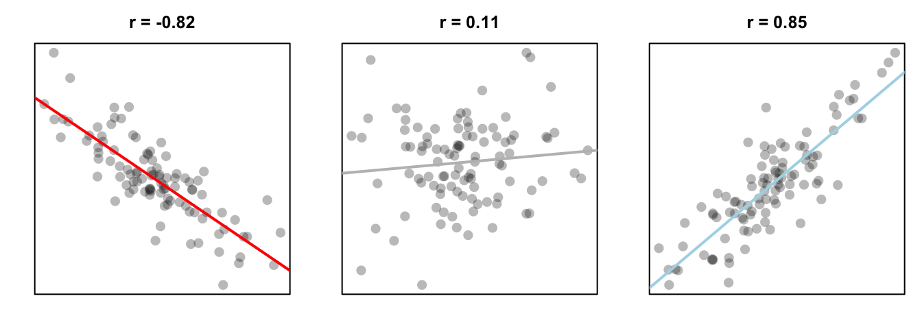
Figure 13.5: Three different correlations. A strong negative correlation, a very small positive correlation, and a strong positive correlation.

To run a correlation test between two variables x and y, use the cor.test() function. You can do this in one of two ways;

if x and y are columns in a dataframe, use the formula notation (formula = ~ x + y).

If x and y are separate vectors (not in a dataframe), use the vector notation (x, y):

Correlation Test - correlating two variables x and y

Method 1: Formula notation - use if x and y are in a dataframe

cor.test(formula = ~ x + y, data = df)

Method 2: Vector notation - use if x and y are separate vectors

cor.test(x = x, y = y)

Just like the t.test() function, we can use the subset argument in the cor.test() function to conduct a test on a subset of the entire dataframe.

Building theory-based methods using computation

As a point of reference, we will now discuss the traditional theory-based way to conduct the hypothesis test for determining if there is a statistically significant difference in the sample mean rating of Action movies versus Romance movies. This method and ones like it work very well when the assumptions are met in order to run the test. They are based on probability models and distributions such as the normal and $t$-distributions.

These traditional methods have been used for many decades back to the time when researchers didn’t have access to computers that could run 5000 simulations in a few seconds. They had to base their methods on probability theory instead. Many fields and researchers continue to use these methods and that is the biggest reason for their inclusion here. It’s important to remember that a $t$-test or a $z$-test is really just an approximation of what you have seen in this chapter already using simulation and randomization. The focus here is on understanding how the shape of the $t$-curve comes about without digging big into the mathematical underpinnings.

Pairwise t-tests

Suppose we have $k$groups of observations. Another approach is to do $(\frac{k}{2})$ t-tests, and adjust the $p$-values for the fact that we are doing multiple t-tests. This has the advantage of showing directly which pairs of groups have significant differences in means, but the disadvantage of not testing directly $H_0:{\mu }_1={\mu }_2=\cdots ={\mu }_k$ versus $H_a:$

at least one of the means is different. See Exercise 6.

For example, returning to the red.cell.folate data, we could do a pairwise t test via the following command:

pairwise.t.test(red.cell.folate$folate, red.cell.folate$ventilation)

## 
##  Pairwise comparisons using t tests with pooled SD 
## 
## data:  red.cell.folate$folate and red.cell.folate$ventilation 
## 
##           N2O+O2,24h N2O+O2,op
## N2O+O2,op 0.042      -        
## O2,24h    0.310      0.408    
## 
## P value adjustment method: holm

We see that there is a significant difference between two of the groups, but not between any of the other pairs. There are several options available with pairwise.t.test, which we discuss below:

1. pool.sd = TRUE can be used when we are assuming equal variances among the groups, and we want to use all of the groups together to estimate the standard deviation. This can be useful if one of the groups is small, for example, but it does require the assumption that the variances of each group is the same.
2. p.adjust.method can be set to one of several options, which can be viewed by typing p.adjust.methods. The easiest to understand is “bonferroni”, which multiplies the $p$

• -values by the number of tests being performed. This is a very conservative adjustment method! The default holm is a good choice. If you wish to compare the results to t.test for diagnostic purposes, then set p.adust.method = "none".
• alternative = "greater" or “less” can be used for one sided-tests. Care must be taken to get the order of the groupings correct in this case.
• var.equal = TRUE can be used if we know the variances are equal, but we do not want to pool the standard deviation. The default is var.equal = FALSE, just like in t.test. This option is not generally recommended.

Conditions for t-test

The infer package does not automatically check conditions for the theoretical methods to work and this warning was given when we used method = "both". In order for the results of the $t$-test to be valid, three conditions must be met:

1. Independent observations in both samples
2. Nearly normal populations OR large sample sizes ($n\ge 30$)

1. Independently selected samples

Condition 1: This is met since we sampled at random using R from our population.

Condition 2: Recall from Figure 10.4, that we know how the populations are distributed. Both of them are close to normally distributed. If we are a little concerned about this assumption, we also do have samples of size larger than 30 ($n_1=n_2=34$).

Condition 3: This is met since there is no natural pairing of a movie in the Action group to a movie in the Romance group.

Since all three conditions are met, we can be reasonably certain that the theory-based test will match the results of the randomization-based test using shuffling. Remember that theory-based tests can produce some incorrect results in these assumptions are not carefully checked. The only assumption for randomization and computational-based methods is that the sample is selected at random. They are our preference and we strongly believe they should be yours as well, but it’s important to also see how the theory-based tests can be done and used as an approximation for the computational techniques until at least more researchers are using these techniques that utilize the power of computers.

Example: $t$-test for two independent samples

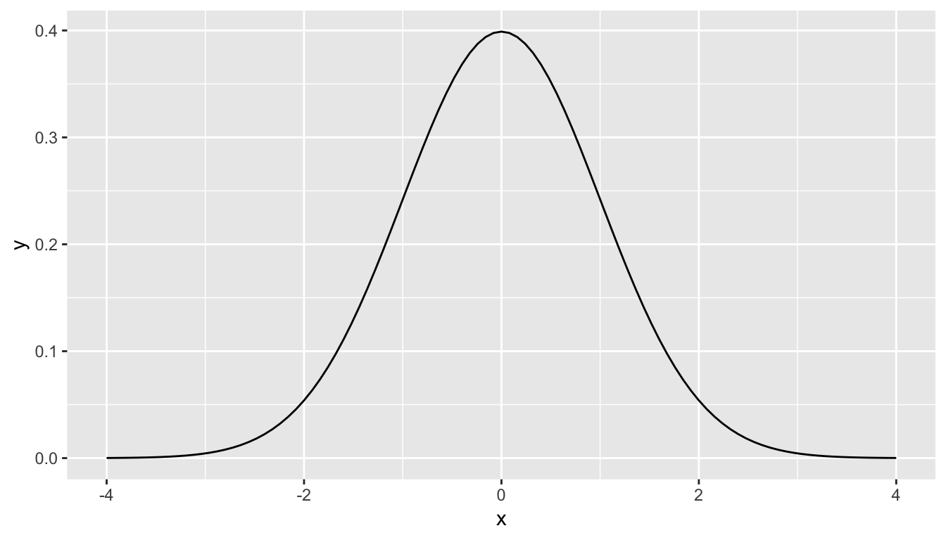
What is commonly done in statistics is the process of normalization. What this entails is calculating the mean and standard deviation of a variable. Then you subtract the mean from each value of your variable and divide by the standard deviation. The most common normalization is known as the $z$-score. The formula for a $z$-score is $$Z=(\frac{x-\mathrm{\mu )/}}{\sigma },$$ where $x$ represent the value of a variable, $\mu$ represents the mean of the variable, and $\sigma$ represents the standard deviation of the variable. Thus, if your variable has 10 elements, each one has a corresponding $z$-score that gives how many standard deviations away that value is from its mean. $z$-scores are normally distributed with mean 0 and standard deviation 1. They have the common, bell-shaped pattern seen below.

Recall that we hardly ever know the mean and standard deviation of the population of interest. This is almost always the case when considering the means of two independent groups. To help account for us not knowing the population parameter values, we can use the sample statistics instead, but this comes with a bit of a price in terms of complexity.

Another form of normalization occurs when we need to use the sample standard deviations as estimates for the unknown population standard deviations. This normalization is often called the $t$-score. For the two independent samples case like what we have for comparing action movies to romance movies, the formula is

There is a lot to try to unpack here.

• ${\overline{x}}_1$is the sample mean response of the first group

• ${\overline{x}}_2$is the sample mean response of the second group
• ${\mu }_1$is the population mean response of the first group
• ${\mu }_2$is the population mean response of the second group
• $s_1$is the sample standard deviation of the response of the first group
• $s_2$is the sample standard deviation of the response of the second group
• $n_1$is the sample size of the first group
• $n_2$is the sample size of the second group

Assuming that the null hypothesis is true ($H_0:{\mu }_1-{\mu }_2=0$), $T$ is said to be distributed following a $t$ distribution with degrees of freedom equal to the smaller value of $n_1-1$ and $n_2-1$. The “degrees of freedom” can be thought of measuring how different the $t$ distribution will be as compared to a normal distribution. Small sample sizes lead to small degrees of freedom and, thus, $t$ distributions that have more values in the tails of their distributions. Large sample sizes lead to large degrees of freedom and, thus, $t$distributions that closely align with the standard normal, bell-shaped curve.

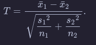
So, assuming $H_0$is true, our formula simplifies a bit:

Heavy tails and outliers

If the results of the preceding section didn’t convince you that you need to understand your underlying population before applying a t-test, then this section will.

A typical “heavy tail” distribution is the $t$ random variable. Indeed, the $t$ rv with 1 or 2 degrees of freedom doesn’t even have a finite standard deviation!

Example

Estimate the effective type I error rate in a t-test of H0:μ=3 versus Ha:μ≠3 at the α=0.1 level when the underlying population is normal with mean 3 and standard deviation 1 with sample size n=100. Assume however, that there is an error in measurement, and one of the values is multiplied by 100 due to a missing decimal point.

mean(replicate(20000, t.test(c(rnorm(99, 3, 1),100*rnorm(1, 3, 1)), mu = 3)$p.value < .1))

These numbers are so small, it makes more sense to sum them:

sum(replicate(20000, t.test(c(rnorm(99, 3, 1),100*rnorm(1, 3, 1)), mu = 3)$p.value < .1))

So, in this example, you see that we would reject H0 3 out of 20,000 times, when the test is designed to reject it 2,000 times out of 20,000! You might as well not even bother running this test, as you are rarely, if ever, going to reject H0 even when it is false.

Rank-based tests

In Chapter 7 we saw how to create confidence intervals and perform hypothesis testing on population means. One of our takeaways, though, was that our techniques were inappropriate to use on populations with big outliers. In this section, we discuss rank based tests that can be used, and are still effective, when the population has these outliers.

One sample Wilcoxon Ranked-Sum Test

In this test, we will be testing $H_0:m=m_0$versus $H_a:m\ne m_0$, where $m$is the median of the underlying population. We will assume that the data is centered symmetrically around the median, so there can be outliers, bimodality or any kind of tails.

Let’s look at how the test works by hand by examining a simple, made up data set. Suppose you wish to test

$$H_0:m=6v\mathrm{s.}$$$$H_a:m\ne 6$$

You collect the data $x_1=15,x_2=7,x_3=3,x_4=10$ and $x_5=13$

. The test works as follows:

1. Compute $y_i=x_i-m_0$for each $i$. We get $y_1=9,y_2=1,y_3=-3,y_4=4$ and $y_5=7$
2. Let $R_i$be the rank of the absolute value of $y_i$. That is, $R_1=5,R_2=1,R_3=2,R_4=3,R_5=4$ since $R_1$ is largest, $R_2$is smallest, etc.
3. Let $r_i$be the signed rank of $R_i$; i.e. $r_i=R_i\times sign\left(y_i\right)$. namely $r_1=5,r_2=1,r_3=-2,r_4=3,r_5=4$
4. Add all of the positive ranks. We get $r_1+r_2+r_4+r_5=13$. That is the test statistic for this test, and it is traditionally called $\mathrm{V.}$
5. Compute the P-value for the test, which is the probability that we get a test statistic $V$which is this, or more, unlikely under the assumption of $H_{0.}$

In order to perform the last step, we need to understand the sampling distribution of $\mathrm{V,}$ under the assumption of the null hypothesis, $H_0$. The ranks of our five data points will always be the numbers 1,2,3,4, and 5. When $H_0$ is true, each data point is equally likely to be positive or negative, and so will be included in the rank-sum half of the time. So, the expected value $$E\left(V\right)=\frac{\mathrm{1/}}{2}\cdot 1+\frac{\mathrm{1/}}{2}\cdot 2+\frac{\mathrm{1/}}{2}\cdot 3+\frac{\mathrm{1/}}{2}\cdot 4+\frac{\mathrm{1/}}{2}\cdot 5=\frac{\mathrm{15/}}{2}=7.5$$ In our example, $V=13$, which is 5.5 away from the expected value of 7.5.

For the probability distribution of $V$, we list all $2^5=32$ possibilities of how the ranks could be signed. Since they are equally likely under $H_0$, we can compute the proportion that lead to a test statistic at least 5.5 away from the expected value of 7.5.

Table 8.1: All possible sums of positive signed ranks

r1	r2	r3	r4	r5	Sum of positive ranks	Far from 7.5?
-1	-2	-3	-4	-5	0	TRUE
-1	-2	-3	-4	5	5	FALSE
-1	-2	-3	4	-5	4	FALSE
-1	-2	-3	4	5	9	FALSE
-1	-2	3	-4	-5	3	FALSE
-1	-2	3	-4	5	8	FALSE
-1	-2	3	4	-5	7	FALSE
-1	-2	3	4	5	12	FALSE
-1	2	-3	-4	-5	2	TRUE
-1	2	-3	-4	5	7	FALSE
-1	2	-3	4	-5	6	FALSE
-1	2	-3	4	5	11	FALSE
-1	2	3	-4	-5	5	FALSE
-1	2	3	-4	5	10	FALSE
-1	2	3	4	-5	9	FALSE
-1	2	3	4	5	14	TRUE
1	-2	-3	-4	-5	1	TRUE
1	-2	-3	-4	5	6	FALSE
1	-2	-3	4	-5	5	FALSE
1	-2	-3	4	5	10	FALSE
1	-2	3	-4	-5	4	FALSE
1	-2	3	-4	5	9	FALSE
1	-2	3	4	-5	8	FALSE
1	-2	3	4	5	13	TRUE
1	2	-3	-4	-5	3	FALSE
1	2	-3	-4	5	8	FALSE
1	2	-3	4	-5	7	FALSE
1	2	-3	4	5	12	FALSE
1	2	3	-4	-5	6	FALSE
1	2	3	-4	5	11	FALSE
1	2	3	4	-5	10	FALSE
1	2	3	4	5	15	TRUE

The last column in Table 8.1 is TRUE if the sum of positive ranks is greater than or equal to 13 or less than or equal to 2. As you can see, we have 6 of the 32 possibilities are at least as far away from the test stat as our data, so the $p$-value would be $\frac{\mathrm{6/}}{32}=.1875$.

Let’s check it with the built in R command.

wilcox.test(c(15,7,3,10,13), mu = 6)

## 
##  Wilcoxon signed rank test
## 
## data:  c(15, 7, 3, 10, 13)
## V = 13, p-value = 0.1875
## alternative hypothesis: true location is not equal to 6

We see that our test statistic V=13 and the p-value is 0.1875, just as we calculated. In general, if you have n data points, the expected value of V is E(V)=n(n+1)/4.

(Exercise 1) To deal with ties, give each data point the average rank of the tied values.

Let’s look at some examples. Consider the react data set. Recall that a t test looks like this:

react <- ISwR::react
t.test(react)

## 
##  One Sample t-test
## 
## data:  react
## t = -7.7512, df = 333, p-value = 1.115e-13
## alternative hypothesis: true mean is not equal to 0
## 95 percent confidence interval:
##  -0.9985214 -0.5942930
## sample estimates:
##  mean of x 
## -0.7964072

and we got a p-value of ${10}^{-13}$. If we instead were to do a wilcoxon test, we get

wilcox.test(react)

## 
##  Wilcoxon signed rank test with continuity correction
## 
## data:  react
## V = 9283.5, p-value = 2.075e-13
## alternative hypothesis: true location is not equal to 0

The p-value is the same order of magnitude, but is closer to double what the other p-value is. Each test is estimating the probability that we will obtain data this far away from $\mu =0$, but they are summarizing what it means to be “this far away from $\mu =0$” in different ways. If the underlying data really is normal, then the t test will be more likely to correctly determine that we can reject $H_0$ when we need to.

Two Sample test

Next, we will be considering wilcox.test when we wish to compare the samples from two distributions (Mann-Whitney-Wilcoxon). We assume that all of the observations are independent for now; in particular, we are assuming we don’t have data that can naturally be matched in pairs (for now).

The null hypothesis is a little complicated to state:

$H_0$: the probability that an observation from sample 1 is larger than an observation from sample 2 is the same as the probability that an observation from sample 2 is larger than an observation from sample 1. That is, $P(X>Y)=P(Y>X)$. We may also rephrase this as a one-sided hypothesis by $P(X>Y)>P(Y>X)$, which would indicate that the values in the first sample are probably larger than the values in the second sample.

The alternative hypothesis is $H_a$$P(X>Y)\ne P(Y>X)$ for the two-sided test, or $P(X>Y)\le P(Y>X)$for the one-sided mentioned above.

The test statistic that we construct is the following: for each data point $x$in Sample 1, we count the number of data points in Sample 2 that are less than $x$. The sum of “wins” is the test statistic. (Count ties as 0.5.) Under the null hypothesis, we expect the test statistic to come out to $$N_1{N}_2/2.$$ The function wilcox.test tells us whether the observed value of the test statistic is far enough away from the expected value to be statistically significant.

Ordinal Data

Another common use of wilcox.test is when the data is ordinal rather than numeric.

Ordinal data is such that given data points $p_1$and $p_2$, we can determine whether $p_1$ is bigger than $p_2$, less than $p_2$, or equal to $p_2$. However, we do not necessarily have a natural way of assigning numbers to the data points. Many people do assume there is a way of assigning numbers to the ordinal categories, but that doesn’t necessarily mean that it is a correct thing to do. For more information, see the somewhat whimsical book Do not use means with Likert scales.

A typical example of ordinal data is Likert-scale data. We have all seen surveys where we are asked to perform tasks such as:

Circle the response that most accurately reflects your opinion

Question	Strongly Agree	Agree	Netural	Disagree	Strongy Disagree
Pride and Prejudice is a great book	1	2	3	4	5
wilcox.test is a useful R command	1	2	3	4	5

Altough the options are listed as numbers, it does not necessarily make sense to treat the responses numerically. For example, if one respondant Strongly Disagrees that wilcox.test is useful, and another Strongly Agrees, is the mean of those responses Neutral? What is the mean of Strongly Agree and Agree? If the responses are numeric, what units do they have? So, it may not (and often does not) make sense to treat the responses to the survey as numeric data, even though it is encoded as numbers. However, we can order the responses in terms of amount of agreement as Strongly Agree > Agree > Disagree > Strongly Disagree. Note that I left out Neutral, because Neutral responses open a whole new can of worms. For example, we don’t know whether someone who put Neutral for Question (1) did so because the have never read Pride and Prejudice, or because they read it and don’t have an opinion on whether it is a great book. In once case, the response might better be treated as missing data, while in the other it would be natural to include the result between Agree and Disagree.

Example

Returning to the movieLens data, the number of stars that a movie receives as a rating can definitely be ordered from 5 stars being the most down to 1/2 star being the least. It is not as clear that the number of stars should be treated numerically, as it is more like asking whether a movie is Very Good, Good, OK, Bad or Very Bad. Consider the movies Toy Story and Toy Story II. Recall that the data that we have in our movie lens data set is a random sample from all users. Is there sufficient evidence to suggest that there is a difference in the ratings of Toy Story and Toy Story II in the full data set?

Before starting, we should decide whether we want to do a one-sided or a two-sided test. Some people have strong opinions about which Toy Story movie is better, but I don’t believe we have sufficient evidence or reason to do a one-sided test. So, let $X$be the rating of Toy Story for a randomly sampled person in the large databaset. Let $Y$be the rating of Toy Story II for a randomly sampled person. Our null and alternative hypotheses are

$H_0:P(X>Y)=P(Y>X)$

$H_a:P(X>Y)\ne P(Y>X)$

In order to do a two-sample Wilcoxon test, we need to load the data.

Discussion

The primary benefit of using wilcox.test versus t.test is that the assumptions that we have made are weaker.

For example, if your data is ordinal rather than numeric, it would not be appropriate to use a t-test without finding a statistically valid way of assigning the ordinal data to numerical values. However, the assumptions on wilcox.test are only that the data points can be compared to determine which is larger, so wilcox.test works just fine with ordinal data.

Wilcox.test in the two sample case is also more resistant to outliers than t.test, just as it is in the one-sample version.

When your underlying data is normal, t.test will be more powerful.

If your underlying data is not skewed, then typically at about 30 samples t.test works pretty well. When data is heavily skewed, you may need up to 100, 500 or even more samples before t.test is accurate.

One down side of wilcox.test is that it is harder to interpret the alternative hypothesis; t.test has a nice, clean statement about the mean, while wilcox.test has a complicated looking statement about probabilities.

Example

This is an example of a paired, one-sided Mann-Whitney-Wilcoxon test. Let’s consider the anorexia data again, which is in the library MASS. We determine whether there is a difference in pre- and post- treatment weight of the subjects who underwent Cognitive Behavioral Treatment. Based on previous work, we expect that CBT will produce an increase in weight, so we use the one-sided test.

$H_0$$P(X>Y)\ge P(Y>X)$

versus

$H_a$: $P(X>Y)<P(Y>X)$.

These are examples of decisions that are made in analyzing data that can have large influences on the outcome of the analysis. It is important to think carefully about your data before going too far in your analysis. If you start playing around with different analyses, looking for one that shows something is significant, then you can end up with drastically underestimated probabilities of Type I errors.

Think about it like this - most every data set has something about it that doesn’t happen too often. If you keep testing until you land on whatever that is, then you have only learned something about the underlying process if your result is reproducible. That’s not to say you can’t look for trends in data; you just need to be sure the trend you find is representative of all data of this type, and can be replicated in further experiments. The more different kinds of analyses you perform before finding something that is significant, the more questionable your result becomes.

Simulations

Here, we see that we correctly reject $H_0$ 78.5% of the time in this simulation. If you repeat the simulations, you will see that indeed the t.test correctly rejects $H_0$more often than the Wilcoxon test does, on average.

However, if there is a departure from normality in the underlying data, Wilcoxon can outperform t.test. Let’s repeat the above simulations in the case that we are sampling from a t distribution with 3 degrees of freedom that has been shifted to the right by one.

Simulating these low probability events is not going to be extremely accurate. but we can say that the probability of getting a result that strong against the null hypothesis by change is very low. If you run the above code several times, you will see that it is between .0002 and .0005; so our estimate for the $p$-value based on this would be that it is somewhere in that range of values. Note that this is different than what wilcox.test returns, in part because we did not take into account ties in our simulation.