Chapter 1.2.3 Expected Value of A Function of An RV: Variance

More generally, one can compute the expected value of a function of a random variable. The formula is

Example Compute $E\left[X^2\right]$ for $X$ that has pmf $p\left(x\right)=(\frac{3}{x})(.5{)}^3$, $x=0,\dots ,3$.

We compute $$E\left[X^2\right]=0^2\times .125+1^2\times .375+2^2\times .375+3^2\times .125=3$$

Example Compute $E\left[X^2\right]$

for $X$ that has pdf $f\left(x\right)=e^{-x}$, $x>0$.

We compute $$E\left[X^2\right]={\int }_0^{\infty }{x}^2{e}^{-x}dx=\left(-x^2{e}^{-x}-2x{e}^{-x}-2e^{-x}\right){|}_0^{\infty }=2$$

(Here, again, we use integration by parts.)

One of the most important examples of expected values of functions of a random variable is the variance of $X$, which is defined by $E\left[\right(X-\mu {)}^2]$, where $\mu =E\left[X\right]$.

Linearity of expected values

We have the following:

$$E[aX+bY]=aE\left[X\right]+bE\left[Y\right]$$

The reason this is true is because of linearity of integration and summation. We will not provide details.

We also have $$E\left[c\right]=\mathrm{c.}$$This is because

$E\left[c\right]=\int cf\left(x\right)dx=c\int f\left(x\right)dx=c$(a similar computation holds for discrete random variables).

Applying linearity of expected values to the definition of variance yields:

$$E\left[\right(X-\mu {)}^2]=E[X^2-2\mu X+{\mu }^2]=E[X^2]-2\mu E[X]+{\mu }^2=E[X^2]-2{\mu }^2+{\mu }^2=$$

$$E\left[X^2\right]-{\mu }^2.$$

This formula for the variance of an rv is often easier to compute than from the definition.

Example

Compute the variance of X if the pdf of X is given by

f(x)=e^(−x), x>0.

We have already seen that E[X] = 1 and E[X^2] = 2.

Therefore, the variance of X is

E[X2]−E[X]2=2−1=1E[X^2] - E[X]^2 = 2 - 1 = 1.

Note that the variance of an rv is always positive (in the French sense¹), as it is the integral (or sum) of a positive function.

Finally, the standard deviation of an rv X is the square root of the variance of X.

Definition

The variance of a random variable X is

The standard deviation of X is the square root of the variance.

The standard deviation is easier to interpret in many cases than the variance. For many distributions, about 95% of the values will lie within 2 standard deviations of the mean. (What do we mean by “about”? Well, 85% would be about 95%. 15% would not be about 95%. It is a very vague rule of thumb. If you want something more precise, see Chebychev’s Theorem, which says in particular that the probability of being more than 2 standard deviations away from the mean is at most 25%.)

Sometimes, you know that the data you collect will likely fall in a certain range of values. For example, if you are measuring the height in inches of 100 randomly selected adult males, you would be able to guess that your data will very likely lie in the interval 60-84.

You can get a rough estimate of the standard deviation by taking the expected range of values and dividing by 6. (Here, we are using the heuristic that “nearly all” data will fall within three standard deviations of the mean.) This can be useful as a quick check on your computations.

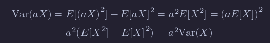
Theorem

Let X and Y be independent random variables, and let a and b be constants. Then,

We will not prove this theorem, but let’s see why the easier statement

Var(aX) = a2Var(X) is true: