Chapter 1.2 Random Variables
Let be the sample space of an experiment. A random variable is a function from to the real line, which is typically denoted by a capital letter. Suppose is a random variable. The expression
denotes the probability that the random variable takes values in the open interval .
This can be done by computing .
(Remember, is a function.)
Example Suppose that three coins are tossed. The sample space is

and all eight outcomes are equally likely, each occurring with probability 1/8. Now, suppose that the number of heads is observed. That corresponds to the random variable which is given by:

In order to compute probabilities, we could use
We will only work explicitly with the sample spaces this one time in this textbook, and we will not always define the sample space when we are defining random variables. It is easier, more intuitive and (for the purposes of this book) equivalent to just understand
for all choices of . In order to understand such probabilities, we will split into two cases.
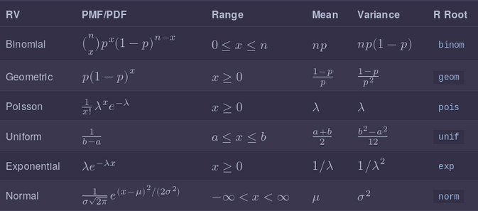
Summary
Here is a list of the (non-optional) random variables that we introduced in this section, together with pmf/pdf, expected value, variance and root R function.
Discrete Random Variables
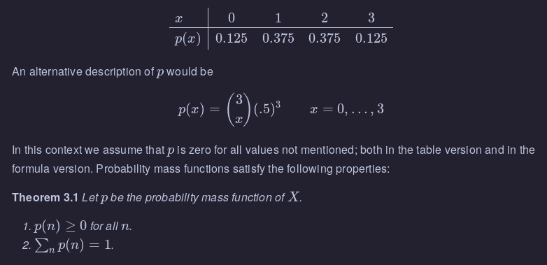
A discrete random variable is a random variable that can only take on values that are integers, or more generally, any discrete subset of . Discrete random variables are characterized by their probability mass function (pmf) . The pmf of a random variable is given by . This is often given either in table form, or as an equation.
Example Let denote the number of Heads observed when a coin is tossed three times. has the following pmf:
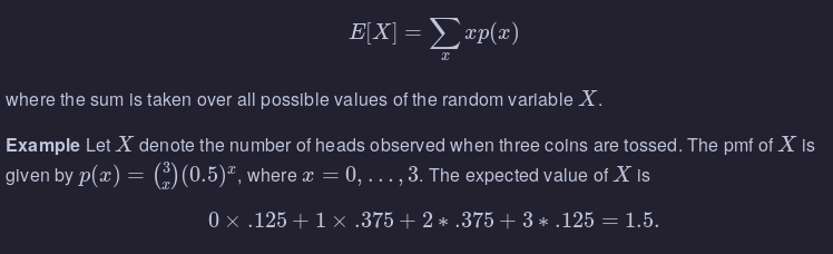
Expected Values of Discrete Random Variables
The expected value of a random variable is, intuitively, the average value that you would expect to get if you observed the random variable more and more times. For example, if you roll a single six-sided die, you would expect the average to be exactly half-way in between 1 and 6; that is, 3.5. The definition is
Continuous Random Variables
A continuous random variable is a random variable for which there exists a function such that whenever (including or )
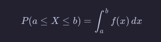
The function in the definition of a continuous random variable is called the probability density function (pdf) of .
The cumulative distribution function (cdf) associated with is the function
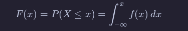
By the fundamental theorem of calculus, is a continuous function, hence the name continuous rv. The function is sometimes referred to as the distribution function of .
One major difference between discrete rvs and continuous rvs is that discrete rv’s can take on only countably many different values, while continuous rvs typically take on values in an interval such as or . Another major difference is that for continuous random variables, for all real numbers .
Theorem
Let be a random variable with pdf and cdf . 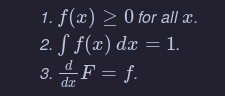
Example Suppose that has pdf for . Find
By definition,
Expected value of a continuous random variable
The expected value of is
Example Find the expected value of when its pdf is given by for .
We compute
(Recall: to integrate you use integration by parts.)
Independent Random Variables
We say that two random variables, X and Y, are independent if knowledge of the outcome of X does not give probabilistic information about the outcome of Y and vice versa. As an example, let X be the amount of rain (in inches) recorded at Lambert Airport on a randomly selected day in 2017, and let Y be the height of a randomly selected person in Botswana. It is difficult to imagine that knowing the value of one of these random variables could give information about the other one, and it is reasonable to assume that the rvs are independent. On the other hand, if X and Y are the height and weight of a randomly selected person in Botswana, then knowledge of one variable could well give probabilistic information about the other. For example, if you know a person is 70 inches tall, it is very unlikely that they weigh 12 pounds.
We would like to formalize that notion by saying that whenever E,F are subsets of R,
P(X∈E|Y∈F)=P(X∈E).
There are several issues with formalizing the notion of independence that way, so we give a definition that is somewhat further removed from the intuition.
The random variables X and Y are independent if
- For all x and y, P(X=x,Y=y)=P(X=x)P(Y=y) if X and Y are discrete.
- For all x and y, P(X≤x,Y≤Y)=P(X≤x)P(Y≤y) if X and Y are continuous.
For our purposes, we will often be assuming that random variables are independent.
Using R to compute probabilities
For all of the random variables that we have mentioned so far (and many more!), R has built in capabilities of computing probabilities. The syntax is broken down into two pieces: the root and the prefix. The root determines which random variable that we are talking about, and here are the names of the ones that we have covered so far:
binomis binomialgeomis geometricpoisis Poissonunifis uniformexpis exponentialnormis normal
The available prefixes are
pcomputes the cumulative distributiondcomputes pdf or pmfrsamples from the rvqquantile function
For now, we will focus on the prefixes p and d.