Chapter 1.2.5.1 Poisson Distribution
Poisson Random Variables
This section discusses the Poisson random variable, which comes from a Poisson process.
Suppose events occur spread over time span [0,T].
If the occurrences of the event satisfy the following properties, then the events form a Poisson process:
- The probability of an event occurring in a time interval [a,b] depends only on the length of the interval [a,b].
- If [a,b] and [c,d] are disjoint time intervals, then the probability that an event occurs in [a,b] is independent of whether an event occurs in [c,d]. (That is, knowing that an event occurred in [a,b] does not change the probability that an event occurs in [c,d].)
- Two events cannot happen at the same time. (Formally, we need to say something about the probability that two or more events happen in the interval [a,a+h] as h→0.)
- The probability of an event occuring in a time interval [a,a+h] is roughly λh, for some constant λ.
Property (4) says that events occur at a certain rate, which is denoted by λ.
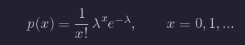
Definition
The pmf of X when X is Poisson with rate λ is
Note that the Taylor series for e^t is ∑n=0∞ 1/n!t^n,
which can be used to show that ∑ xp(x) = 1.
Theorem
Example
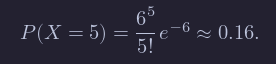
Suppose a typist makes typos at a rate of 3 typos per page. What is the probability that they will make exactly 5 typos on a two page sample?
Here, we assume that typos follow the properties of a Poisson rv. It is not clear that they follow it exactly. For example, if the typist has just made a mistake, it is possible that their fingers are no longer on home position, which means another mistake is likely, violating the independence rule (2). Nevertheless, assuming the typos are Poisson is a reasonable approximation.
The rate at which typos occur per two pages is 6, so we use λ = 6 in the formula for Poisson. We get
Using R, and the pdf dpois:
dpois(5,6)## [1] 0.1606231There is a 0.16 probability of making exactly five typos on a two-page sample.
Often, when modeling a count of something, you need to choose between binomial, geometric, and Poisson.
The binomial and geometric random variables both come from Bernoulli trials, where there is a sequence of individual trials each resulting in success or failure.
In the Poisson process, events are spread over a time interval, and appear at random.
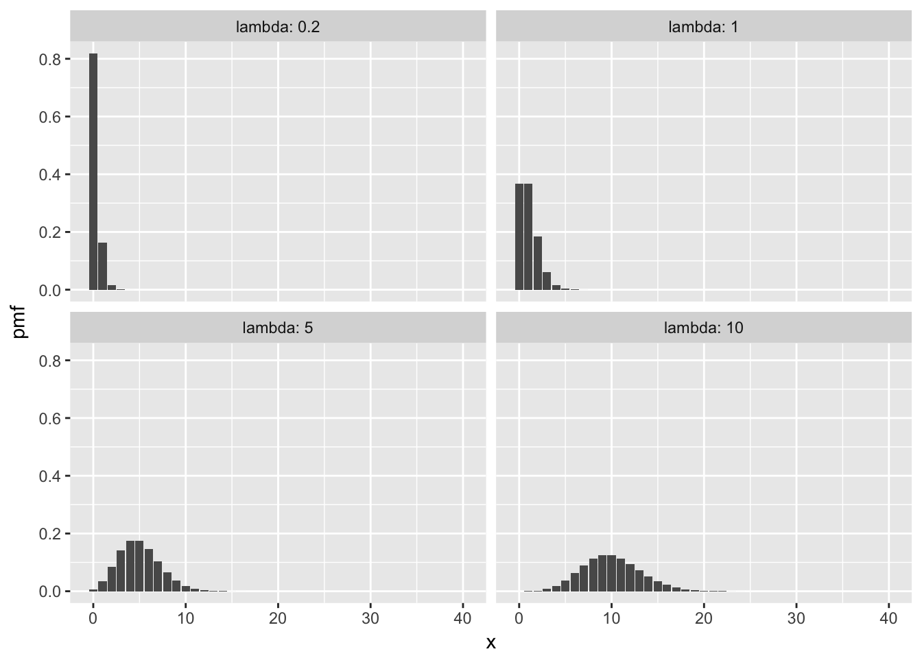
Here some plots of pmfs with various means.
Poisson Random Variables and Experiments
- Definition: Poisson Distribution is a discrete probability distribution that expresses the probability of the number of events occurring in a fixed period of time. These events occur with a known average rate and are independent of the time since the last event. The Poisson Distribution can also be used for the number of events in other specified intervals such as distance, area or volume.
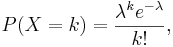
- Mass function: For X~Poisson(λ), the Poisson mass function is given by
 where
where
- e is the natural number (e = 2.71828...)
- k is the number of occurrences of an event - the probability of which is given by the mass function

- λ is a positive real number, equal to the expected number of occurrences that occur during the given interval. For instance, if the events occur on average every 4 minutes, and you are interested in the number of events occurring in a 10 minute interval, you would use as model a Poisson distribution with λ=10/4=2.5.
- Notes
- The Poisson Distribution can be derived as a limiting case of the Binomial Distribution.
- The Poisson Distribution can be applied to systems with a large number of possible events, each of which is rare. A classic example is the nuclear decay of atoms and Positron Emission Tomography Imaging.
- Expectation: The expected value of a Poisson distributed random variable X is λ.
- Variance: The Poisson variance is λ.
- Example: See this SOCR Poisson distribution activity.
Example
Suppose one expects to see 40 shooting stars per hour at night (by observing at a specific location and not using visual enhancers). Assume that the process of observing arrivals (shooting stars) is Poisson(λ = 40).
- Compute the probability that in a 1 hour timeframe, the number of observed shooting stars will be between 44 and 52! We can compute this as follows: Let
 .
.
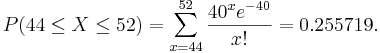 The figure below shows this result using SOCR distributions:

- Note: We observe that this distribution is bell-shaped. We can also use the Normal distribution to approximate this probability. Using
 , together with the continuity correction for better approximation we obtain
  , which is close to the exact that was found earlier. The figure below shows this probability.

Applications
The Poisson Distribution arises in many different discrete situations when the probability of the observed phenomenon is constant in time or space. Examples of events that may be modeled by Poisson Distribution include:
- The number of cars that pass through a certain point on a road (sufficiently distant from traffic lights) during a given period of time.
- The number of spelling mistakes one makes while typing a single page.
- The number of phone calls at a call center per minute.
- The number of times a web server is accessed per minute.
- The number of road kill (animals killed) found per unit length of road.
- The number of mutations in a given stretch of DNA after a certain amount of radiation exposure.
- The number of unstable atomic nuclei that decayed within a given period of time in a piece of radioactive substance.
- The number of pine trees per unit area of mixed forest.
- The number of stars in a given volume of space.
- The distribution of visual receptor cells in the retina of the human eye.
- The number of light bulbs that burn out in a certain amount of time.
- The number of viruses that can infect a cell in cell culture.
- The number of hematopoietic stem cells in a sample of unfractionated bone marrow cells.
- The number of inventions of an inventor over their career.
- The number of particles that "scatter" off of a target in a nuclear or high energy physics experiment.
Poisson as a Limiting Case of Binomial Distribution
In several of the above examples, the events being counted are actually the outcomes of discrete trials, and would more precisely be modeled using the Binomial Distribution with parameters n (number of trials) and  (probability of success). That is, Binomial(n,p) approaches the Poisson(λ) distribution, where expected value
  , as n approaches infinity. This provides the means to approximate Binomial random variables (for large n) using the Poisson distribution. The details of this approximation are below:
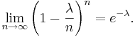
Let  and
and  . Then we have


- As
 the first term approaches 1; the second remains constant since "n" does not appear in it at all; the third approaches e-λ; and the fourth expression approaches 1.
- Consequently the limit is

More generally, whenever a sequence of binomial random variables with parameters n and pn is such that
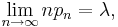
the sequence converges (in distribution) to a Poisson random variable with mean λ.