Chapter 1.2.4 Simulation of RVs

In this chapter we discuss simulation related to random variables. We will simulate probabilities related to random variables, and more importantly for our purposes, we will simulate pdfs and pmfs of random variables.

Estimating probabilities of rvs via simulation

In order to run simulations with random variables, we will use the R command r + distname, where distname is the name of the distribution, such as unif, geom, pois, norm, exp or binom.

The first argument to any of these functions is the number of samples to create.

Most distname choices can take additional arguments that affect their behavior. For example, if I want to create a random sample of size 100 from a normal random variable with mean 5 and sd 2, I would use rnorm(100,5,2). Without the additional arguments, rnorm gives the standard normal random variable, with mean 0 and sd 1. For example, rnorm(10000) gives 10000 random values of the standard normal random variable $Z$ .

Theorems about transformations of random variables

In this section, we will be estimating the pdf of transformations of random variables and comparing them to known pdfs. The goal will be to find a known pdf that closely matches our estimate, so that we can develop some theorems.

Example

Compare the pdf of $2Z$ , where $Z\simNormal(0,1)$ to the pdf of a normal random variable with mean 0 and standard deviation 2.

We already saw how to estimate the pdf of $2Z$ , we just need to plot the pdf of $Normal(0,2)$ on the same graph.

The pdf $f(x)$ of $Normal(0,2)$ is given in R by the function $f(x)=dnorm(x,0,2)$ .

We can add the graph of a function to a ggplot using the stat_function command.

zData <- 2 * rnorm(10000)
f <- function(x) dnorm(x,0,2)
ggplot(data.frame(zData), aes(x = zData)) + 
  geom_density() + 
  stat_function(fun = f,color="red")

Wow! Those look really close to the same thing!

Theorem

Let

X

be a normal random variable with mean

μ

and standard deviation

σ

. Then,

aX+b

is a normal random variable with mean

aμ+b

and standard deviation

aσ

Example

Let $Z$ be a standard normal rv. Find the pdf of $Z^2$ and compare it to the pdf of a $χ2$ (chi-squared) rv with one degree of freedom.

The distname for a $χ2$ rv is chisq, and rchisq requires the degrees of freedom to be specified using the df parameter.

We plot the pdf of $Z^2$ and the chi-squared rv with one degree of freedom on the same plot. $χ2$ with one df has a vertical asymptote at $x=0$ , so we need to explicitly set the $y$ -axis scale:

zData <- rnorm(10000)^2
f <- function(x) dchisq(x, df=1)
ggplot(data.frame(zData), aes(x = zData)) +
  coord_cartesian(ylim = c(0,1.2)) +        # set y-axis scale
  geom_density() + 
  stat_function(fun = f, color = "red")

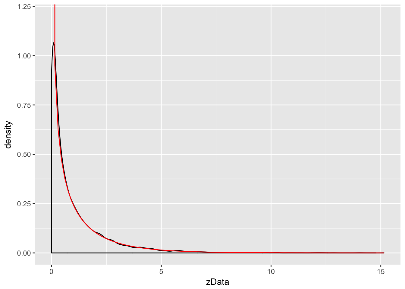
As you can see, the estimated density follows the true density quite well. This is evidence that $Z^2$ is, in fact, chi-squared.

Theorem: Let

Z

be a normal random variable with mean 0 and standard deviation 1. Then,

Z^2

is a chi-squared random variable with 1 degree of freedom.

The Central Limit Theorem

Let

X1,\dots,Xn

be iid (independent and identically distributed) rvs with mean

μ

and standard deviation

σ

Then

(X¯-μ) / (σ/sqrt(n)) \to Z as n\to\infty

where

Z

is a standard normal rv.

We will not prove this theorem, but we will do simulations for several examples. They will all follow a similar format.

The Central Limit Theorem says that, if you take the mean of a large number of independent samples, then the distribution of that mean will be approximately normal.

We call $X¯$ the sample mean because it is the mean of a random sample. In practice, if the population you are sampling from is symmetric with no outliers, then you can start to see a good approximation to normality after as few as 15-20 samples. If the population is moderately skew, such as exponential or $χ2$ , then it can take between 30-50 samples before getting a good approximation. Data with extreme skewness, such as some financial data where most entries are 0, a few are small, and even fewer are extremely large, may not be appropriate for the central limit theorem even with 500 samples (see example below). Finally, there are versions of the central limit theorem available when the $Xi$ are not iid, but a single outlier of sufficient size invalidates the hypotheses of the Central Limit Theorem, and $X¯$ will not be normally distributed.