Chapter 6.2.3 ANOVA

In the last chapter we covered 1 and two sample hypothesis tests. In these tests, you are either comparing 1 group to a hypothesized value, or comparing the relationship between two groups (either their means or their correlation).

In this chapter, we’ll cover how to analyse more complex experimental designs with ANOVAs.

When do you conduct an ANOVA? You conduct an ANOVA when you are testing the effect of one or more nominal (aka factor) independent variable(s) on a numerical dependent variable.

A nominal (factor) variable is one that contains a finite number of categories with no inherent order. Gender, profession, experimental conditions, and Justin Bieber albums are good examples of factors (not necessarily of good music). If you only include one independent variable, this is called a One-way ANOVA. If you include two independent variables, this is called a Two-way ANOVA. If you include three independent variables it is called a Menage a trois `NOVA.

What does ANOVA stand for?

ANOVA stands for “Analysis of variance.” At first glance, this sounds like a strange name to give to a test that you use to find differences in means, not differences in variances. However, ANOVA actually uses variances to determine whether or not there are ‘real’ differences in the means of groups. Specifically, it looks at how variable data are within groups and compares that to the variability of data between groups. If the between-group variance is large compared to the within group variance, the ANOVA will conclude that the groups do differ in their means. If the between-group variance is small compared to the within group variance, the ANOVA will conclude that the groups are all the same. See Figure~ for a visual depiction of an ANOVA.

Question	Analysis	Formula
Is there a difference between the different cleaners on cleaning time (ignoring poop type)?	One way ANOVA	`time ~ cleaner`
Is there a difference between the different poop types on cleaning time (ignoring which cleaner is used)	One-way ANOVA	`time ~ type`
Is there a unique effect of the cleaner or poop types on cleaning time?	Two-way ANOVA	`time ~ cleaner + type`
Does the effect of cleaner depend on the poop type?	Two-way ANOVA with interaction term	`time ~ cleaner * type`

Full-factorial between-subjects ANOVA

There are many types of ANOVAs that depend on the type of data you are analyzing. In fact, there are so many types of ANOVAs that there are entire books explaining differences between one type and another.

For this book, we’ll cover just one type of ANOVAs called full-factorial, between-subjects ANOVAs. These are the simplest types of ANOVAs which are used to analyze a standard experimental design.

In a full-factorial, between-subjects ANOVA, participants (aka, source of data) are randomly assigned to a unique combination of factors – where a combination of factors means a specific experimental condition. For example, consider a psychology study comparing the effects of caffeine on cognitive performance. The study could have two independent variables: drink type (soda vs. coffee vs. energy drink), and drink dose (.25l, .5l, 1l). In a full-factorial design, each participant in the study would be randomly assigned to one drink type and one drink dose condition. In this design, there would be 3 x 3 = 9 conditions.

For the rest of this chapter, I will refer to full-factorial between-subjects ANOVAs as `standard’ ANOVAs.

Repeated measures ANOVA using the lme4 package

If you are conducting an analyses where you’re repeating measurements over one or more third variables, like giving the same participant different tests, you should do a mixed-effects regression analysis. To do this, you should use the lmer function in the lme4 package. For example, in our poopdeck data, we have repeated measurements for days. That is, on each day, we had 6 measurements. Now, it’s possible that the overall cleaning times differed depending on the day. We can account for this by including random intercepts for day by adding the (1|day) term to the formula specification. For more tips on mixed-effects analyses, check out this great tutorial by Bodo Winter at http://www.bodowinter.com/tutorial/bw_LME_tutorial2.pdf.

Comparing regression models with `anova()`

A good model not only needs to fit data well, it also needs to be parsimonious. That is, a good model should be only be as complex as necessary to describe a dataset. If you are choosing between a very simple model with 1 IV, and a very complex model with, say, 10 IVs, the very complex model needs to provide a much better fit to the data in order to justify its increased complexity. If it can’t, then the more simpler model should be preferred.

To compare the fits of two models, you can use the anova() function with the regression objects as two separate arguments. The anova() function will take the model objects as arguments, and return an ANOVA testing whether the more complex model is significantly better at capturing the data than the simpler model. If the resulting p-value is sufficiently low (usually less than 0.05), we conclude that the more complex model is significantly better than the simpler model, and thus favor the more complex model. If the p-value is not sufficiently low (usually greater than 0.05), we should favor the simpler model.

Setup

Notation

$x_{i j}$ denotes the $j$ th observation from the $i$ th group.
${\bar{x}}_{i \cdot}$ denotes the mean of the observations in the $i$ th group.
${\bar{x}}_{\cdot}$ denotes the mean of all observations.

As an example, in red.cell.folate, there are 3 groups. We have $x_{11} = 243, x_{12} = 251, \dots, x_{21} = 206, \dots, x_{31} = 241, \dots .$

To compute the group means:

red.cell.folate %>% group_by(ventilation) %>% summarize(mean(folate))

## # A tibble: 3 x 2
##   ventilation `mean(folate)`
##        <fctr>          <dbl>
## 1  N2O+O2,24h       316.6250
## 2   N2O+O2,op       256.4444
## 3      O2,24h       278.0000

This tells us that ${\bar{x}}_{1 \cdot} = 316.625$ , for example.

To get the overall mean, we use mean(red.cell.folate$folate), which is 283.2.

Our model for the folate level is

$x_{i j} = μ + α_{i} + ϵ_{i j},$

where $μ$ is the grand mean, $α_{i}$ represents the difference between the grand mean and the group mean, and $ϵ_{i j}$ represents the variation within the group.

So, each individual data point could be realized as

$x_{i j} = {¯ ¯ ¯ x}_{\cdot} + ({¯ ¯ ¯ x}_{i \cdot} - ¯ ¯ ¯ x) + (x_{i j} - {¯ ¯ ¯ x}_{i \cdot})$

The null hypothesis for ANOVA is that the group means are all equal (or equivalently all of the $α_{i}$ are zero). So, if $μ_{i} = μ + α_{i}$ is the true group mean, we have:

H0:μ1=μ2=⋯=μk
Ha:Not all μi are equal

An alternative test statistic

We considered the t test statistic as a way to evaluate the strength of evidence for a hypothesis test in Section 5.4.3. However, we could focus on R**2. Recall that R**2 described the proportion of variability in the response variable (y) explained by the explanatory variable (x). If this proportion is large, then this suggests a linear relationship exists
between the variables. If this proportion is small, then the evidence provided by the data may not be convincing.

This concept – considering the amount of variability in the response variable explained by the explanatory variable – is a key component in some statistical techniques.

The analysis of variance (ANOVA) technique introduced in Section 4.4 uses this general principle. The method states that if enough variability is explained away by the categories, then we would conclude the mean varied between the categories. On the other hand, we might not be convinced if only a little variability is explained. ANOVA can be further employed in advanced regression modeling to evaluate the inclusion of explanatory variables.

ANOVA is “analysis of variance” because we will compare the variation of data within individual groups with the overall variation of the data.

We make assumptions (below) to predict the behavior of this comparison when $H_{0}$ is true. If the observed behavior is unlikely, it gives evidence against the null hypothesis. The general idea of comparing variance within groups to the variance between groups is applicable in a wide variety of situations.

Define the variation within groups to be $S S D_{W} = \sum i \sum j (x_{i j} - {¯ ¯ ¯ x}_{i \cdot})^{2}$

and the variation between groups to be $S S D_{B} = \sum i \sum j ({¯ ¯ ¯ x}_{i \cdot} - ¯ ¯ ¯ x)^{2}$

and the total variation to be $S S D_{t o t} = \sum i \sum j (¯ ¯ ¯ x - x_{i j})^{2} .$

Theorem

With the above notation,

$S S D_{t o t} = S S D_{W} + S S D_{B}$

This says that the total variation can be broken down into the variation between groups plus the variation within the groups.

If the variation between groups is much larger than the variation within groups, then that is evidence that there is a difference in the means of the groups.

The question then becomes: how large is large? In order to answer that, we will need to examine the SSDB and SSDW terms more carefully. At this point, we also will need to make

Assumptions

The population is normally distributed within each group
The variances of the groups are equal.

Notation We have $k$ groups. There are $n_{i}$ observations in group $i$ , and $N = \sum n_{i}$ total observations.

Notice that $S S D_{W}$ is almost $\sum \sum ({\bar{x}}_{i j} - μ_{i})^{2}$ , in which case $S S D_{W} / σ^{2}$ would be a $χ^{2}$ random variable with $N$ degrees of freedom.

However, we are making $k$ replacements of means by their estimates, so we subtract $k$ to get that $S S D_{B} / σ^{2}$ is $χ^{2}$ with $N - k$ degrees of freedom. (This follows the heuristic we started in Section 4.6.2).

As for $S S D_{B}$ , it is trickier to see, but $\sum_{i} \sum_{j} (x_{i \cdot} - μ)^{2} / σ^{2}$ would be $χ^{2}$ with $k$ degrees of freedom. Replacing $μ$ by $\bar{x}$ makes $S S D_{B} / σ^{2}$ a $χ^{2}$ rv with $k - 1$ degrees of freedom.

The test statistic for ANOVA is:

$F = \frac{S S D_{B} / (σ^{2} (k - 1)) /}{S S D_{W} / (σ^{2} (N - k))}$

$= \frac{S S D_{B} / (k - 1) /}{S S D_{W} / (N - k)}$

This is the ratio of two χ2 rvs divided by their degrees of freedom; hence, it is F with k−1 and N−k degrees of freedom.

Through this admittedly very heuristic derivation, you can see why we must assume that we have equal variances (otherwise we wouldn’t be able to cancel the unknown σ2) and normality (so that we get a known distribution for the test statistic).

If F is much bigger than 1, then we reject H0:μ1=μ2=⋯=μk in favor of the alternative hypothesis that not all of the μi are equal.

4 Steps to conduct an ANOVA

Here are the 4 steps you should follow to conduct a standard ANOVA in R:

Create an ANOVA object using the aov() function. In the aov() function, specify the independent and dependent variable(s) with a formula with the format y ~ x1 + x2 where y is the dependent variable, and x1, x2 … are one (more more) factor independent variables.

# Step 1: Create an aov object
mod.aov <- aov(formula = y ~ x1 + x2 + ...,
               data = data)

Create a summary ANOVA table by applying the summary() function to the ANOVA object you created in Step 1.

# Step 2: Look at a summary of the aov object
summary(mod.aov)

If necessary, calculate post-hoc tests by applying a post-hoc testing function like TukeyHSD() to the ANOVA object you created in Step 1.

# Step 3: Calculate post-hoc tests
TukeyHSD(mod.aov)

If necessary, interpret the nature of the group differences by creating a linear regression object using lm() using the same arguments you used in the aov() function in Step 1.

# Step 4: Look at coefficients
mod.lm <- lm(formula = y ~ x1 + x2 + ...,
             data = data)

summary(mod.lm)

I almost always find it helpful to combine an ANOVA summary table with a regression summary table.

Because ANOVA is just a special case of regression (where all the independent variables are factors), you’ll get the same results with a regression object as you will with an ANOVA object. However, the format of the results are different and frequently easier to interpret.

To create a regression object, use the lm() function. Your inputs to this function will be identical to your inputs to the aov() function.

Type I, Type II, and Type III ANOVAs

It turns out that there is not just one way to calculate ANOVAs. In fact, there are three different types - called, Type 1, 2, and 3 (or Type I, II and III). These types differ in how they calculate variability (specifically the sums of of squares).

If your data is relatively balanced, meaning that there are relatively equal numbers of observations in each group, then all three types will give you the same answer.

However, if your data are unbalanced, meaning that some groups of data have many more observations than others, then you need to use Type II (2) or Type III (3).

The standard aov() function in base-R uses Type I sums of squares. Therefore, it is only appropriate when your data are balanced.

If your data are unbalanced, you should conduct an ANOVA with Type II or Type III sums of squares. To do this, you can use the Anova() function in the car package. The Anova() function has an argument called type that allows you to specify the type of ANOVA you want to calculate.

In the next code chunk, I’ll calculate 3 separate ANOVAs from the poopdeck data using the three different types. First, I’ll create a regression object with lm(). As you’ll see, the Anova() function requires you to enter a regression object as the main argument, and not a formula and dataset. That is, you need to first create a regression object from the data with lm() (or glm()), and then enter that object into the Anova() function. You can also do the same thing with the standard aov() function.

# Step 1: Calculate regression object with lm()
time.lm <- lm(formula = time ~ type + cleaner,
              data = poopdeck)

Now that I’ve created the regression object time.lm, I can calculate the three different types of ANOVAs by entering the object as the main argument to either aov() for a Type I ANOVA, or Anova() in the car package for a Type II or Type III ANOVA:

# Type I ANOVA - aov()
time.I.aov <- aov(time.lm)

# Type II ANOVA - Anova(type = 2)
time.II.aov <- car::Anova(time.lm, type = 2)

# Type III ANOVA - Anova(type = 3)
time.III.aov <- car::Anova(time.lm, type = 3)

As it happens, the data in the poopdeck dataframe are perfectly balanced (so we’ll get exactly the same result for each ANOVA type. However, if they were not balanced, then we should not use the Type I ANOVA calculated with the aov() function.

To see if your data are balanced, you can use the function:

# Are observations in the poopdeck data balanced?
with(poopdeck,
     table(cleaner, type))
##        type
## cleaner parrot shark
##       a    100   100
##       b    100   100
##       c    100   100

As you can see, in the poopdeck data, the observations are perfectly balanced, so it doesn’t matter which type of ANOVA we use to analyse the data.

For more detail on the different types, check out https://mcfromnz.wordpress.com/2011/03/02/anova-type-iiiiii-ss-explained/.

Examples

red.cell.folate

Returning to red.cell.folate, we use R to do all of the computations for us.

First, build a linear model for folate as explained by ventilation, and then apply the anova function to the model. anova produces a table which contains all of the computations from the discussion above.

rcf.mod <- lm(folate~ventilation, data = red.cell.folate)
anova(rcf.mod)

## Analysis of Variance Table
## 
## Response: folate
##             Df Sum Sq Mean Sq F value  Pr(>F)  
## ventilation  2  15516  7757.9  3.7113 0.04359 *
## Residuals   19  39716  2090.3                  
## ---
## Signif. codes:  0 '***' 0.001 '**' 0.01 '*' 0.05 '.' 0.1 ' ' 1

The two rows ventilation and Residuals correspond to the between group and within group variation.

The first column, Df gives the degrees of freedom in each case. Since $k = 3$ , the between group variation has $k - 1 = 2$ degrees of freedom, and since $N = 22$ , the within group variation (Residuals) has $N - k = 19$ degrees of freedom.

The Sum Sq column gives $S S D_{B}$ and $S S D_{W}$ .

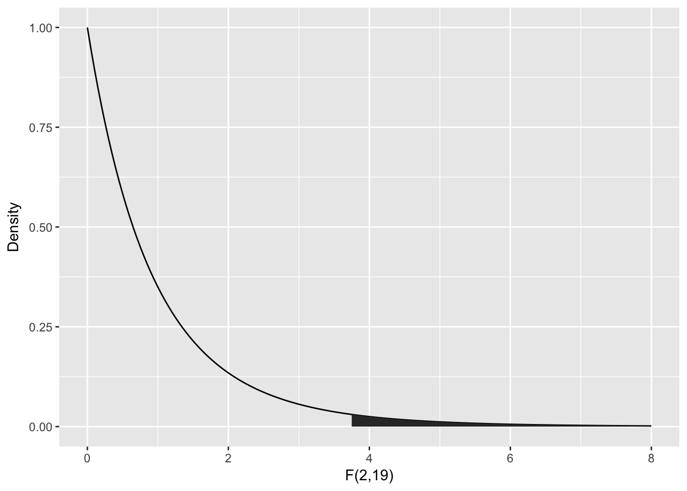
The Mean Sq variable is the Sum Sq value divided by the degrees of freedom. These two numbers are the numerator and denominator of the test statistic, $F$ . So here, $F = 7757.9 / 2090.3 = 3.7113$ .

To compute the $p$ -value, we need the area under the tail of the $F$ distribution above $F = 3.7113$ . Note that this is a one-tailed test, because small values of $F$ would actually be evidence in favor of $H_{0}$ .

One-way ANOVA

In this chapter, we introduce one-way analysis of variance (ANOVA) through the analysis of a motivating example.
Consider the red.cell.folate data in ISwR. We have data on folate levels of patients under three different treatments. Suppose we want to know whether treatment has a significant effect on the folate level of the patient. How would we proceed? First, we would want to plot the data. A boxplot is a good idea.

library(ISwR)
library(ggplot2)
red.cell.folate <- ISwR::red.cell.folate
ggplot(red.cell.folate, aes(x = ventilation, y = folate)) +
geom_boxplot()

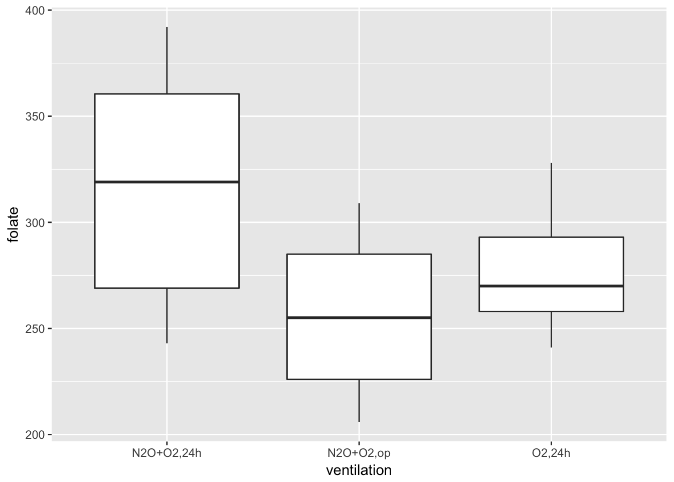
Looking at this data, it is not clear whether there is a difference. It seems that the folate level under treatment 1 is perhaps higher. We could try to compare the means of each pair of ventilations using t.test(). The problem with that is we would be doing three tests, and we would need to adjust our p-values accordingly. We are going to take a different approach, which is ANOVA.

Two-way ANOVA - interactions

Interactions between variables test whether or not the effect of one variable depends on another variable. For example, we could use an interaction to answer the question: Does the effect of cleaners depend on the type of poop they are used to clean? To include interaction terms in an ANOVA, just use an asterix (*) instead of the plus (+) between the terms in your formula. Note that when you include an interaction term in a regression object, R will automatically include the main effects as well/

Center variables before computing interactions!

# Create a regression model with interactions between 
#   IVS weight and clarity
diamonds.int.lm <- lm(formula = value ~ weight * clarity,
                      data = diamonds)

# Show summary statistics of model coefficients
summary(diamonds.int.lm)$coefficients
##                Estimate Std. Error t value  Pr(>|t|)
## (Intercept)    157.4721     10.569 14.8987 4.170e-31
## weight           0.9787      1.070  0.9149 3.617e-01
## clarity          9.9245     10.485  0.9465 3.454e-01
## weight:clarity   1.2447      1.055  1.1797 2.401e-01

Hey what happened? Why are all the variables now non-significant? Does this mean that there is really no relationship between weight and clarity on value after all? No. Recall from your second-year pirate statistics class that when you include interaction terms in a model, you should always center the independent variables first. Centering a variable means simply subtracting the mean of the variable from all observations.