Chapter 2.1.4 Data Frames

There are two important S3 vectors that are built on top of lists: data frames and tibbles.

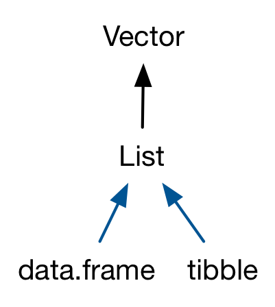
Data frames are used to store tabular data in R. They are an important type of object in R and are used in a variety of statistical modeling applications. Hadley Wickham’s package dplyr has an optimized set of functions designed to work efficiently with data frames.

Data frame is a two dimensional data structure in R. Since a data frame is a list of vectors, it is possible for a data frame to have a column that is a list. Data frames are represented as a special type of list where every element of the list has to have the same length. Each element of the list can be thought of as a column and the length of each element of the list is the number of rows.

Unlike matrices, data frames can store different classes of objects in each column. Matrices must have every aelement be the same class (e.g. all integers or all numeric).

This is very useful because a list can contain any other object, which means that you can put any object in a data frame. This allows you to keep related objects together in a row, no matter how complex the individual objects are. You can see an application of this in the “Many Models” chapter of “R for Data Science”, http://r4ds.had.co.nz/many-models.html.

List columns

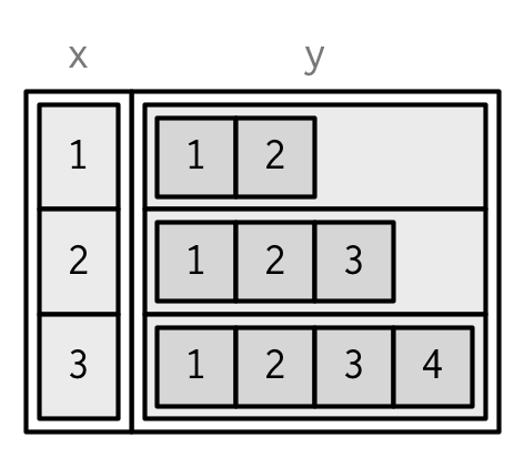
List-columns are allowed in data frames but you have to do a little extra work, either adding the list-column after creation, or wrapping the list in I().

List-columns are allowed in data frames but you have to do a little extra work, either adding the list-column after creation, or wrapping the list in I().




df <- data.frame(x = 1:3)
df$y <- list(1:2, 1:3, 1:4)

data.frame(
x = 1:3, 
y = I(list(1:2, 1:3, 1:4))
)
#> x y
#> 1 1 1, 2
#> 2 2 1, 2, 3
#> 3 3 1, 2, 3, 4

Matrix and data frame columns

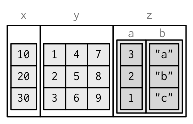
It’s also possible to have a column of a data frame that’s a matrix or array, as long as the number of rows matches the data frame. (This requires a slight extension to our definition of a data frame: it’s not the length() of each column that must be equal; but the NROW().) Like with list-columns, you must either add after creation, or wrap in I().

dfm <- data.frame(
x = 1:3 * 10
)
dfm$y <- matrix(1:9, nrow = 3)
dfm$z <- data.frame(a = 3:1, b = letters[1:3], stringsAsFactors = FALSE)

str(dfm)
#> 'data.frame': 3 obs. of 3 variables:
#> $ x: num 10 20 30
#> $ y: int [1:3, 1:3] 1 2 3 4 5 6 7 8 9
#> $ z:'data.frame': 3 obs. of 2 variables:
#> ..$ a: int 3 2 1
#> ..$ b: chr "a" "b" "c"

Data frames are one of the biggest and most important ideas in R, and one of the things that makes R different from other programming languages. However, in the over 20 years since their creation, the ways people use R have changed, and some of the design decisions that made sense at the time data frames were created now cause frustration.

This frustration lead to the creation of the tibble (Müller and Wickham 2018), a modern reimagining of the data frame.

Tibbles are designed to be (as much as possible) drop-in replacements for data frames, while still fixing the greatest frustrations. A concise and fun way to summarise the main differences is that tibbles are lazy and surly: they tend to do less and complain more.

Data frames are usually created by reading in a dataset using the read.table() or read.csv(). However, data frames can also be created explicitly with the data.frame() function or they can be coerced from other types of objects like lists.

Data frames can be converted to a matrix by calling data.matrix(). While it might seem that the as.matrix() function should be used to coerce a data frame to a matrix, almost always, what you want is the result of data.matrix().

Check if a variable is a data frame or not:

We can check if a variable is a data frame or not using the class() function.

Many data input functions of R like, read.table(), read.csv(), read.delim(), read.fwf() also read data into a data frame.

In the following you’ll learn about data frames in R; how to create them, access their elements and modify them in your program.

How to access Components of a Data Frame?

Components of data frame can be accessed like a list or like a matrix.

Accessing like a list

We can use either [, [[ or $ operator to access columns of data frame.

Accessing like a matrix

Data frames can be accessed like a matrix by providing index for row and column.

To illustrate this, we use datasets already available in R. Datasets that are available can be listed with the command library(help = "datasets").

A data frame can be examined using functions like str() and head().

How to modify a Data Frame in R?

Data frames can be modified like we modified matrices through reassignment.

Adding Components

Rows can be added to a data frame using the rbind() function. Similarly, we can add columns using cbind().

Exploring data frames

Among the many ways of getting a feel for the data contained in a data frame such as flights, we present three functions that take as their argument the data frame in question:

Using the View() function built for use in RStudio. We will use this the most.
Using the glimpse() function loaded via dplyr package
Using the kable() function in the knitr package
Using the $ operator to view a single variable in a data frame

`View()`

Run View(flights) in your Console in RStudio and explore this data frame in the resulting pop-up viewer. You should get into the habit of always Viewing any data frames that come your way.

Note the capital “V” in View. R is case-sensitive so you’ll receive an error is you run view(flights) instead of View(flights).

By running View(flights), we see the different variables listed in the columns and we see that there are different types of variables. Some of the variables like distance, day, and arr_delay are what we will call quantitative variables. These variables are numerical in nature. Other variables here are categorical.

Note that if you look in the leftmost column of the View(flights) output, you will see a column of numbers. These are the row numbers of the dataset. If you glance across a row with the same number, say row 5, you can get an idea of what each row corresponds to. In other words, this will allow you to identify what object is being referred to in a given row. This is often called the observational unit.

The observational unit in this example is an individual flight departing New York City in 2013. You can identify the observational unit by determining what the thing is that is being measured in each of the variables.

`glimpse()`

The second way to explore a data frame is using the glimpse() function that you can access after you’ve loaded the dplyr package. It provides us with much of the above information and more.

We see that glimpse will give you the first few entries of each variable in a row after the variable. In addition, the data type (See Subsection 2.2.1) of the variable is given immediately after each variable’s name inside < >. Here, int and num refer to quantitative variables. In contrast, chr refers to categorical variables. One more type of variable is given here with the time_hour variable: dttm. As you may suspect, this variable corresponds to a specific date and time of day.

`kable()`

The final way to explore the entirety of a data frame is using the kable() function from the knitr package. Let’s explore the different carrier codes for all the airlines in our dataset two ways. Run both of these in your Console:

airlines
kable(airlines)

At first glance of both outputs, it may not appear that there is much difference. However, we’ll see later on, especially when using a tool for document production called R Markdown, that the latter produces output that is much more legible.

`$` operator

Lastly, the $ operator allows us to explore a single variable within a data frame. For example, run the following in your console

airlines
airlines$name

We used the $ operator to extract only the name variable and return it as a vector of length 16. We will only be occasionally exploring data frames using this operator.

Row names

In addition to column names, indicating the names of the variables or predictors, data frames have a special attribute called row.names which indicate information about each row of the data frame.

Because each element of the list has the same length, data frames have a rectangular structure, and hence shares properties of both the matrix and the list:

A data frame has 1d names(), and 2d colnames() and rownames()¹⁸. The names() and colnames() are identical.
A data frame has 1d length(), and 2d ncol() and nrow(). The length() is the number of columns.

Row names arise naturally if you think of data frames as 2d structures like matrices: the columns (variables) have names so the rows (observations) should too. Most matrices are numeric, so having a place to store character labels is important. But this analogy to matrices is misleading because matrices possess an important property that data frames do not: they are transposable. In matrices the rows and columns are interchangeable, and transposing a matrix gives you another matrix (and transposing again gives you back the original matrix). With data frames, however, the rows and columns are not interchangeable, and the transpose of a data frame is not a data frame.

There are three reasons that row names are suboptimal:

Metadata is data, so storing it in a different way to the rest of the data is fundamentally a bad idea. It also means that you need to learn a new set of tools to work with row names; you can’t use what you already know about manipulating columns.
Row names are poor abstraction for labelling rows because they only work when a row can be identified by a single string. This fails in many cases, for example when you want to identify a row by a non-character vector (e.g. a time point), or with multiple vectors (e.g. position, encoded by latitude and longitude).
Row names must be unique, so any replication of rows (e.g. from bootstrapping) will create new row names. If you want to match rows from before and after the transformation you’ll need to perform complicated string surgery.

For these reasons, tibbles do not support row names. Instead the tibble package provides tools to easily convert row names into a regular column with either rownames_to_column(), or the rownames argument to as_tibble().

Printing

One of the most obvious differences between tibbles and data frames is how they are printed.

Tibbles:

Only show the first 10 rows and all the columns that will fit on screen. Additional columns are shown at the bottom.
Each column is labelled with its type, abbreviated to three or four letters.
Wide columns are truncated to avoid a single long string occupying an entire row. (This is still a work in progress: it’s tricky to get the tradeoff right between showing as many columns as possible and showing a single wide column fully.)
When used in console environments that support it, colour is used judiciously to highlight important information, and de-emphasise supplemental details.